Environmental noise efects on entanglement fidelity of exchange-coupled semiconductor spin qubits

Throckmorton et al., arXiv:1610.02032 (2016) 的机器可读全文页。

文献信息

Throckmorton et al., arXiv:1610.02032 (2016)，“Environmental noise efects on entanglement fidelity of exchange-coupled semiconductor spin qubits”. arXiv:1610.02032 · DOI:10.1103/physrevb.95.085405 原文为 arXiv 预印本版本的机器可读转换，公式与图注以原文为准；本页仅作站内索引与全文查阅，引用请以正式出版物为准。

全文

Environmental noise efects on entanglement fidelity of exchange-coupled semiconductor spin qubits

Robert E. Throckmorton,¹ Edwin Barnes,^{1, 2} and S. Das Sarma¹

¹Condensed Matter Theory Center and Joint Quantum Institute, Department of Physics,

University of Maryland, College Park, Maryland 20742-4111 USA

²Department of Physics, Virginia Tech, Blacksburg, Virginia 24061, USA

(Dated: February 8, 2017)

We investigate the efect of magnetic field and charge noise on the generation of entanglement between two Heisenberg exchange-coupled electron spins in a double quantum dot. We focus on exchange-driven evolution that would ideally take an initial unentangled tensor product state to a maximally-entangled state in the absence of noise. The presence of noise obviously adversely afects the attainment of maximal entanglement, which we study quantitatively and exactly. To quantify the efects of noise, we calculate two-qubit coherence times and entanglement fidelity, both of which can be extracted from simulations or measurements of the return probability as a function of interaction time, i.e., the time period during which the exchange coupling remains efective between the two spins. We perform these calculations for a broad range of noise strengths that includes the regime of recent experiments. We find that the two types of noise reduce the amount of entanglement in qualitatively distinct ways and that, although charge noise generally leads to faster decoherence, the relative importance of the two types of noise in entanglement creation depends sensitively on the strength of the exchange coupling. Our results can be used to determine the level of noise suppression needed to reach quantum error correction thresholds. We provide quantitative guidance for the requisite noise constraints necessary to eventually reach the > 99% fidelity consistent with the quantum error correction threshold.

I. INTRODUCTION

Electron spins in semiconductor quantum dots are an attractive platform for quantum computation for two rea sons. One is the simple fact that this platform is compatible with the existing semiconductor electronics industry, making scalability much more feasible¹. The other is the possibility of faster operations compared to other platforms, such as trapped ions or atoms and qubits based on superconducting circuits. These advantages have provided the impetus behind the substantial theoretical and experimental progress on GaAs- and Si-based systems that has been made over the past decade. High-fidelity single-qubit gates and control over multiqubit arrays have been demonstrated in several diferent types of spin qubits, including single-spin Loss-DiVincenzo qubits^2–8, double-dot singlet-triplet qubits^9–15, triple-dot exchangeonly qubits^16–20, and hybrid qubits^21–23 consisting of three electrons confined in a double quantum dot.

Universal quantum computation requires not only high-fidelity initialization, readout, and single-qubit gates, but two-qubit entangling gates as well. While there has also been progress in achieving the latter^24–28, with two-qubit gate fidelities as high as 90% reported in recent work²⁸, fidelities have not yet reached the thresholds necessary for quantum error correction schemes²⁹. This is due in large part to decoherence caused by environmental noise. The two main sources of noise are magnetic field noise, hereafter referred to simply as field noise, due to both nuclear spins in the host semiconductor (Overhauser noise)³⁰ and fluctuations in the applied magnetic field, and charge noise due to charge fluctuations on nearby impurities or on the electrostatic gates used to confine electrons, leading to noise in the exchange coupling between the spins³¹. Field noise is especially large in GaAs; in fact, it is the dominant source of noise in this material and cannot be eliminated as the only stable isotopes of Ga and As have nonzero nuclear spin. However, its efects can be considerably reduced by dynamical decoupling^32–35 or Bayesian estimation of Hamiltonian parameters^13,36. On the other hand, field noise is less of a problem in Si; of the three stable isotopes, only ²⁹Si has a nonzero nuclear spin, and the concentration of this isotope can be greatly reduced via isotopic purification³⁷. However, charge noise continues to be a serious problem in Si, and the field noise arising from fluctuations in the applied magnetic field remains an issue.

Developing a theoretical understanding of the efects of noise on entanglement creation in a system of two spin qubits is therefore of great importance for future progress in building a semiconductor-based quantum computer. However, a systematic investigation of the efects of both field and charge noise on our ability to create entanglement has not been conducted previously. A number of works have introduced dynamical noise-suppression techniques, such as the dynamical decoupling and Bayesian estimation methods mentioned above, as well as dynamically corrected gates^38–46, which partially cancel out the efects of noise by applying carefully designed pulse sequences. In addition, several works have studied the decoherence of an initially prepared entangled state of two or more qubits subject to various types of noise^47–51. There has also been some theoretical work on the dy namics of two coupled electron spins under a constant exchange coupling and applied magnetic field gradient. Two early treatments^52,53 mostly focused on field noise, but included a limited discussion of charge noise as well. In more recent works, we have studied the efects of noise on single-qubit coherence⁵⁴ and on the state preservation of two exchange-coupled qubits⁵⁵. However, none of these works provides a comprehensive analysis of how noise limits entanglement generation in two-spin-qubit systems subject to realistic noise. The question of how much noise is tolerable in the implementation of twoqubit gates at the error correction threshold remains unknown. The goal of the present work is to address this question, which is obviously of vital importance if semiconductor spin quantum computing is going to be a practical reality in the future.

Most of the aforementioned works make use of the quasistatic bath approximation⁵⁶ in which the noise is modeled by averaging the return probability over a Gaussian distribution of magnetic fields and exchange couplings. It is well known that the actual field and charge noise in spin qubit experiments both have a complicated frequency dependence. Much work has been devoted to measuring this dependence^14,58 since it plays an important role in experiments that study or manipulate spin evolution over time scales exceeding a few hundred nanoseconds. On the other hand, for experiments that focus on shorter time scales, the Gaussian quasistatic model has been shown to work well in fitting experimental ${\mathrm{data}}^{15,19,54,57}$ . Since our focus here is on characterizing the efects of noise in these types of experiments, we employ the quasistatic model throughout this work. While a detailed investigation of the efects of frequency-dependent noise is important, it is beyond the scope of our present work.

The objective of our work is to calculate the fidelity of entanglement generation of two Heisenberg-coupled electron spins in the presence of field and charge noise, starting from the “classical” unentangled state . Suppose we allow the system to evolve from this initial state under the Heisenberg Hamiltonian with no magnetic field gradient, i.e., under the influence of the exchange coupling $J$ alone. In the complete absence of noise, the system will evolve into one of two maximally entangled states, $\begin{array}{r}|M{E}_1⟩=\frac{1}{\sqrt{2}}(|\uparrow \downarrow ⟩-i|\downarrow \uparrow ⟩)\end{array}$ ) and $\begin{array}{r}|M{E}_2⟩=\frac{1}{\sqrt{2}}(|\bar{\uparrow }\downarrow ⟩+i|\downarrow \uparrow ⟩)\end{array}$ ), after times $t=\pi /2J$ and $t=3\pi /2J_{:}$ , respectively. The fidelities for producing these states are closely related to an intrinsic two-qubit coherence time, which we denote by $T_2^{\ast }$ , and to the steady-state return probability. We emphasize that this $T_2^{\ast }$ , to be defined precisely in Sec. IIB below, is not the same as the free induction decay time for a single electron spin—this is a two-electron property (the 2 in the subscript of $T_2^{\ast }$ here refers to two qubits or two coupled spins) that measures the suppression of entanglement creation between the two qubits. For the ideal entangling operation, the return probability oscillates in time about $\frac{1}{2}$ with an amplitude of $\frac{1}{2}$ . Both the average (steady-state) value and the amplitude of oscillations are important for quantifying the maximum amount of entanglement that can be generated. The intrinsic coherence time is a measure of the decay rate of the oscillation amplitude of the return probability under the influence of disorder, and is thus a measure of the time scale over which one can maximally entangle two electron spins. The steady-state value of the return probability can also be influenced by noise, and deviations away from $\frac{1}{2}$ will lead to a further, time-independent reduction of entanglement. Our results can be used to determine to what extent the noise must be reduced in order to achieve two-qubit entanglement fidelities that exceed quantum error correction thresholds. We also calculate the fidelities for producing the states, $|M{E}_1⟩$ and $|M{E}_2⟩$ , which are defined as the disorder-averaged probabilities that, after performing the operations that, ideally, would evolve the system from the unentangled state to these maximally entangled states, we will measure the system to be in the appropriate state^59,60.

Our main findings are as follows. We find that the coherence time decreases as we increase either type of noise, but that charge noise has a noticeably greater efect. As a very important check, we find that, in the absence of magnetic disorder, the coherence time is inversely proportional to the charge noise strength for low disorder, in agreement with the quasistatic bath approximation ${\lfloor }^{56}$ ; the fact that this is only approximate in our case is due to the fact that we only allow for positive exchange coupling strengths, consistent with the experimental situation in exchange-coupled semiconductor spin systems. We also find that, in general, in the complete absence of field noise, the steady-state return probability is always $\begin{array}{l}\frac{1}{2}\end{array}$ . This means that one can still achieve maximal entanglement as long as the operation is done over a time scale much shorter than $T_2^{\ast }$ . If there is any field noise, however, then the steady-state return probability is larger than $\frac{1}{2},$ leading to a reduction in the entanglement fidelity regardless of how quickly the entanglement is generated. Our results for the entangled state fidelities follow a somewhat diferent trend to that of $T_2^{\ast }-$ —we find that whereas $T_2^{\ast }$ is much more sensitive to charge noise than field noise, the entanglement fidelity for preparing state $|M{E}_1⟩$ is essentially equally sensitive to both types of noise. On the other hand, the fidelity for preparing $|M{E}_2⟩$ is afected less by field noise than by charge noise. This follows from the basic observation that it takes three times longer to prepare $|M{E}_2⟩$ combined with the fact that charge noise tends to dominate on longer time scales. We note that similar analytic results to those that we find here are obtained for a triple quantum dot system in Ref. 61.

Although these results would suggest that, in theory, charge noise would generally be a more severe problem for realizing a maximally entangled state than field noise, we should note that, as mentioned before, field noise tends to be much larger than charge noise in actual experiments, at least in $\mathrm{GaAs},$ meaning that field noise is the dominant cause of decoherence and thus loss of entanglement fidelity by the simple virtue of being the dominant source of noise in the system. However, it is possible to mitigate the efects of field noise by increasing the exchange coupling. If we quantify the strengths of the two types of noise present in the system by the standard deviations of their respective distributions, ${\sigma }_h$ for field noise and ${\sigma }_J$ for charge noise, then we will find that all of the quantities we calculate depend on the noise strengths only in the dimensionless combinations, ${\sigma }_h/J_0$ and ${\sigma }_J/J_0$ , where $J_0$ is the mean of the exchangecoupling distribution. It has been shown that as $J_0$ is increased, ${\sigma }_h$ remains approximately constant, while ${\sigma }_J$ increases roughly linearly.⁵⁴ Thus, even though field noise is strong in GaAs, it is possible to mitigate its efects by simply increasing the exchange coupling, leaving charge noise as the main contributor to loss of entanglement fidelity. This observation suggests that comparable entanglement fidelities can be achieved in both GaAs and Si systems, even when isotopic purification is employed in the latter case, as one can reduce the efective dimensionless field noise even in GaAs simply by increasing the exchange coupling strength. Of course, single-qubit operations (i.e., spin rotations) are also directly afected by field noise, but powerful dynamical decoupling techniques could mitigate field noise efects on single qubit operations. In the current work, we focus entirely on twoqubit exchange gate operations as the subject of single qubit operations for semiconductor spin qubit systems have already been studied rather exhaustively both theoretically and experimentally with single qubit fidelity already reaching 99% in some situations.

The rest of the paper is organized as follows. In Sec. II, we review the Heisenberg Hamiltonian from which our results ultimately derive, review the known results for the eigenstates, eigenenergies, and return probability, and define the disorder average and intrinsic coherence time. Section III is dedicated to our main results for the steady-state return probability, coherence time, and fidelity. We first give results in the limits of no field noise and no charge noise, showing that we can obtain some purely analytical results in these limits. We then give our exact numerical results for the general case in which both types of noise are present. We give our conclusions in Sec. IV.

II. MODEL AND DEFINITIONS

In this section, we review the Hamiltonian and eigen states of the two-spin Heisenberg model, as well as the return probability and magnetization for the system starting from a “classical” unentangled state. We also give our definition of the intrinsic coherence time, $T_2^{\ast }$ which we will be using throughout this paper.

A. Heisenberg Hamiltonian

Our Hamiltonian is that of two electron spins coupled via a disordered Heisenberg exchange coupling subject to magnetic fields^52,53,55:

$$H=J{\vec{S}}_1\cdot {\vec{S}}_2+h_1{S}_{1,z}+h_2{S}_{2,z}.\text{\hspace{1em}(1)}$$

Here, we take the magnetic fields $h_1$ and $h_2$ to have Gaussian distributions with a mean of $h_0$ and standard devi ation ${\sigma }_h$ , hereafter called the “strength” of the disorder,

$$f_{h_i}(h_i)=\frac{1}{{\sigma }_h\sqrt{2\pi }}{e}^{-(h_i-h_0{)}^2/2{\sigma }_h^2},\text{\hspace{1em}(2)}$$

and the exchange coupling to have a truncated Gaussian distribution $(i.e.$ , we restrict J to non-negative values) with a mean of $J_0$ and standard deviation ${\sigma }_J$ ,

$$f_J(J)=\frac{1}{{\sigma }_J\sqrt{2\pi }}\frac{2}{1+\mathrm{erf}\left(\frac{J_0}{{\sigma }_J\sqrt{2}}\right)}{e}^{-(J-J_0{)}^2/2{\sigma }_J^2}.\text{\hspace{1em}(3)}$$

This Hamiltonian conserves the z component of the total spin, $S_z=S_{1,z}+S_{2,z};$ we will focus on the $S_z=0$ subspace from this point on, as there is only one eigenstate in each of the $S_z=\pm 1$ subspaces, and therefore the dynamics of the system within these subspaces will be trivial.

The efective Hamiltonian describing the $S_z=0$ subspace is

$$H_{\mathrm{eff}}=\frac{1}{2}J{\sigma }_x+\frac{1}{2}\delta h{\sigma }_z-\frac{1}{4}J,\text{\hspace{1em}(4)}$$

where $\delta h:=:h_1:-:h_2$ This Hamiltonian is written in the and $|\downarrow \uparrow ⟩$ basis, with the former being the ${{}^{64}\mathrm{top}}^7$ component of our spinors. Our subsequent calculations will be simplified by noting that the distribution of δh is also Gaussian, with zero mean and standard deviation ${\sigma }_h\sqrt{2}$ :

$$f_{\delta h}(\delta h)=\frac{1}{2{\sigma }_h\sqrt{\pi }}{e}^{-(\delta h{)}^2/4{\sigma }_h^2}.\text{\hspace{1em}(5)}$$

Diagonalizing the efective Hamiltonian^52,53,55, one finds that the energy eigenvalues are

$$E_{\pm }=-\frac{1}{4}J\pm \frac{1}{2}\sqrt{J^2+(\delta h{)}^2},\text{\hspace{1em}(6)}$$

and the associated eigenstates are

$${\psi }_{\pm }=\left[\begin{array}{l}\frac{1}{\sqrt{2}}\sqrt{1\pm \frac{\delta h}{\sqrt{J^2+(\delta h{)}^2}}}\\ \pm \frac{1}{\sqrt{2}}\sqrt{1\mp \frac{\delta h}{\sqrt{J^2+(\delta h{)}^2}}}\end{array}\right].\text{\hspace{1em}(7)}$$

Let us now consider initializing the system in the state. We now give the result for the return probability, $P_{\uparrow \downarrow }(t)=|⟨\uparrow \downarrow |\downarrow \breve{\Psi (t)}⟩{|}^2$ , which is^53,55

$$P_{\uparrow \downarrow }(t)=1-\frac{J^2}{J^2+(\delta h{)}^2}{\sin }^2\left[\frac{1}{2}\sqrt{J^2+(\delta h{)}^2}t\right].\text{\hspace{1em}(8)}$$

We denote the disorder average of a quantity A as $[A{]}_{\alpha }$ 2 which is defined simply as

$$[A{]}_{\alpha }={\int }_{-\infty }^{\infty }d(\delta h){\int }_0^{\infty }dJ{f}_{\delta h}(\delta h)f_J(J)A.\text{\hspace{1em}(9)}$$

In general, this average must be evaluated numerically; however, as we will see below, there are special cases in which it is possible to obtain analytical results.

B. Definition of $T_2^{\ast }$

We now define the intrinsic coherence time, $T_2^{\ast }$ . We will see below that the disorder-averaged return probability shows oscillations that decay in amplitude, tending toward a steady-state value. We define $T_2^{\ast }$ as the time that it takes for the amplitude of these oscillations about the steady-state value to decay to $1/e$ times the initial amplitude. We wish to emphasize two points about $T_2^{\ast }$ First, this definition is purely operational—it is independent of the detailed time dependence of the amplitude and is used purely for convenience. Any other reasonable definition of $T_2^{\ast }$ will result in the same conclusions. Second, $T_2^{\ast }$ here is not related to the free-induction decay time of a single qubit—rather, it is a two-qubit property, as already emphasized in Sec. I. It is a measure of the rate at which our ability to entangle the two qubits is suppressed as the time scale of entanglement generation is increased. Also note that the dimensionless number ${\mathcal{J}}_0{\mathcal{T}}_2^{\ast }$ gives the number of coherent oscillations exhibited in the return probability before it decays.

We may connect this decay of the oscillation amplitude of the return probability to entanglement of the two electron spins as follows. Let us first consider the case with no noise and no magnetic field gradient. In this case, we find that the return probability is just the oscillatory function,

$$P_{\uparrow \downarrow }(t)=\frac{1+\cos Jt}{2}.\text{\hspace{1em}(10)}$$

We therefore see that the return probability oscillates around $\frac{1}{2}$ with an amplitude of $\begin{array}{l}\frac{1}{2}\end{array}$ . If we let the system evolve for a time $t=\pi /2J$ , then the return probability will be exactly $\frac{1}{2}$ , while the state of the system will be the maximally entangled state,

$$e^{-i\pi {\sigma }_x/4}|\uparrow \downarrow ⟩=\frac{1}{\sqrt{2}}(|\uparrow \downarrow ⟩-i|\downarrow \uparrow ⟩)=|M{E}_1⟩,\text{\hspace{1em}(11)}$$

which difers from the singlet and triplet states by only single-qubit operations. We may also realize a maximally entangled state by evolving the system for a time $t:=$ 3π $/2\bar{J};$ in this case, we obtain

$$e^{-3i\pi {\sigma }_x/4}|\uparrow \downarrow ⟩=-\frac{1}{\sqrt{2}}(|\uparrow \downarrow ⟩+i|\downarrow \uparrow ⟩)=-|M{E}_2⟩.\text{\hspace{1em}(12)}$$

We thus see that a return probability of the form given in Eq. (10) indicates an operation that is capable of producing a maximally entangled state. These operations are in fact $\sqrt{\mathrm{SWAP}}$ gates up to single-qubit rotations. Any deviations from this form, whether due to the amplitude decaying or due to a shift in the value about which the probability oscillates, indicate a reduction in our ability to produce such maximal entanglement. Therefore, one may view $T_2^{\ast }$ as an operationally defined characteristic time scale over which the two-qubit entanglement decays.

III. RETURN PROBABILITY AND COHERENCE TIME

We now present our results for the disorder-averaged return probability $[P_{\uparrow \downarrow }(t){]}_o$ and the intrinsic coherence times $T_2^{\ast }$ extracted from it. We first present the general formula for the return probability, and then show that, in the ${\sigma }_h=0$ and ${\sigma }_J=0$ limits, we can obtain some closed-form analytical results.

If we substitute $Eq.(8)$ into $Eq.(9)$ , use the trigonometric identity, si $1^2\dot{\theta }=\frac{\dot{1}-\cos 2\theta }{2}$ , and rewrite in terms of the real part of a complex-valued expression, we obtain

$$\begin{array}{rl}[P_{\uparrow \downarrow }(t){]}_{\alpha }& =1-\frac{1}{2\pi {\sigma }_h{\sigma }_J\sqrt{2}\left[1+\mathrm{erf}\left(\frac{J_0}{{\sigma }_J\sqrt{2}}\right)\right]}{\int }_{-\infty }^{\infty }d(\delta h){\int }_0^{\infty }dJ\frac{J^2}{J^2+(\delta h{)}^2}{e}^{-(\delta h{)}^2/4{\sigma }_h^2}{e}^{-(J-J_0{)}^2/2{\sigma }_J^2}\\ & +\frac{1}{2\pi {\sigma }_h{\sigma }_J\sqrt{2}\left[1+\mathrm{erf}\left(\frac{J_0}{{\sigma }_J\sqrt{2}}\right)\right]}\mathrm{Re}\left[{\int }_{-\infty }^{\infty }d(\delta h){\int }_0^{\infty }dJ\frac{J^2}{J^2+(\delta h{)}^2}{e}^{-(\delta h{)}^2/4{\sigma }_h^2}{e}^{-(J-J_0{)}^2/2{\sigma }_{\mathcal{J}}^2}{e}^{i\sqrt{J^2+(\delta h{)}^2}t}\right].\end{array}\text{\hspace{1em}(13)}$$

We now show that the first two terms of the above expression give the steady-state return probability, which we will denote by $P_S.$ , so that all of the oscillations about said steady-state value come from the third term. Let us denote the integral in the third term by $I(t)$ :

$$\begin{array}{l}I(t)={\int }_{-\infty }^{\infty }d(\delta h){\int }_0^{\infty }dJ\frac{J^2}{J^2+(\delta h{)}^2}{e}^{-(\delta h{)}^2/4{\sigma }_h^2}\\ \times e^{-(J-J_0{)}^2/2{\sigma }_J^2}{e}^{i\sqrt{J^2+(\delta h{)}^2}t}\end{array}\text{\hspace{1em}(14)}$$

If we rewrite this in polar coordinates, $\delta h=r\cos \theta$ and

J = r sin θ, we obtain

$$\begin{array}{rl}I(t)& =2{\int }_0^{\infty }dr{\int }_0^{\pi /2}d\theta r{\sin }^2\theta e^{-r^2{\cos }^2\theta /4{\sigma }_h^2}\\ & \times e^{-(r\sin \theta -J_0{)}^2/2{\sigma }_J^2}{e}^{irt}.\end{array}\text{\hspace{1em}(15)}$$

We now take the Fourier transform,

$$I(\omega )={\int }_{-\infty }^{\infty }dtI(t)e^{-i\omega t},\text{\hspace{1em}(16)}$$

of this expression, obtaining, for $\omega \ge 0$ 2

$$\begin{array}{rl}I(\omega )& =2{\int }_0^{\infty }dr{\int }_0^{\pi /2}d\theta r{\sin }^2\theta e^{-r^2{\cos }^2\theta /4{\sigma }_h^2}\\ & \times e^{-(r\sin \theta -J_0{)}^2/2{\sigma }_J^2}\cdot 2\pi \delta (\omega -r)\\ & =4\pi \omega {\int }_0^{\pi /2}d\theta {\sin }^2\theta e^{-{\omega }^2{\cos }^2\theta /4{\sigma }_h^2}{e}^{-(\omega \sin \theta -J_0{)}^2/2{\sigma }_J^2}\end{array}\text{\hspace{1em}(17)}$$

We thus see that $I(\omega =0)=0$ , and thus the third term in $[P_{\uparrow \downarrow }(t){]}_{\alpha }$ simply represents oscillations about the steadystate value, which is given by the first two terms:

$$\begin{array}{l}{P}_S=1-\frac{1}{2\pi {\sigma }_h{\sigma }_J\sqrt{2}\left[1+\mathrm{erf}\left(\frac{J_0}{{\sigma }_J\sqrt{2}}\right)\right]}\\ \times {\int }_{-\infty }^{\infty }d(\delta h){\int }_0^{\infty }dJ\frac{J^2}{J^2+(\delta h{)}^2}{e}^{-(\delta h{)}^2/4{\sigma }_h^2}\\ \times e^{-(J-J_0{)}^2/2{\sigma }_J^2}.\end{array}\text{\hspace{1em}(18)}$$ $$\mathbf{A}.{\sigma }_h=0\text{ limit }$$

Now we turn our attention to the ${\sigma }_h=0$ limit. In this case, the steady-state return probability is just

$$\begin{array}{l}{P}_S=1-\frac{1}{{\sigma }_J\sqrt{2\pi }\left[1+\mathrm{erf}\left(\frac{J_0}{{\sigma }_J\sqrt{2}}\right)\right]}{\int }_0^{\infty }dJ{e}^{-(J-J_0{)}^2/2{\sigma }_J^2}\\ =\frac{1}{2}.\end{array}\text{\hspace{1em}(19)}$$

We can also obtain a closed-form analytical solution for the return probability as a function of time. Our formula for $\left[P_{\uparrow \downarrow }(t)\right]$ α becomes

$$\begin{array}{l}[P_{\uparrow \downarrow }(t){]}_{\alpha }=\frac{1}{2}+\frac{1}{{\sigma }_J\sqrt{2\pi }\left[1+\mathrm{erf}\left(\frac{J_0}{{\sigma }_J\sqrt{2}}\right)\right]}\\ \times \mathrm{Re}\left[{\int }_0^{\infty }dJ{e}^{-(J-J_0{)}^2/2{\sigma }_J^2}{e}^{iJt}\right].\end{array}\text{\hspace{1em}(20)}$$

The integral can be evaluated analytically in terms of the error function; we obtain

$$[P_{\uparrow \downarrow }(t){]}_{\alpha }=\frac{1}{2}+\frac{1}{2\left[1+\mathrm{erf}\left(\frac{J_0}{{\sigma }_J\sqrt{2}}\right)\right]}{e}^{-{\sigma }_J^2{t}^2/2}$$ $$\times \left\{\cos J_{0}t+\mathrm{Re}\left[e^{i{J}_{0}t}\mathrm{erf}\left(\frac{J_0}{{\sigma }_J\sqrt{2}}+i\frac{{\sigma }_{J}t}{\sqrt{2}}\right)\right]\right\}.\text{\hspace{1em}(21)}$$

We now show that, in the limit, ${\sigma }_J\ll J_0$ , it is possible to obtain an approximate analytical expression for $T_2^{\ast }$ In this limit, we may drop the imaginary part of the argument of the error function, obtaining

$$[P_{\uparrow \downarrow }(t){]}_{\alpha }\approx \frac{1}{2}(1+e^{-{\sigma }_J^2{t}^2/2}\cos J_{0}t).\text{\hspace{1em}(22)}$$

This approximation only holds if $\begin{array}{r}t\ll \frac{J_0}{{\sigma }_T^2}\end{array}$ . We see that, in this limit, the return probability has a Gaussian decay towards its steady-state value. We can now simply read of the value of $T_2^{\ast }$ , obtaining

$$T_2^{\ast }\approx \frac{\sqrt{2}}{{\sigma }_J}.\text{\hspace{1em}(23)}$$

For small ${\sigma }_J\left(\ll J_0\right)$ , we thus see that our approximation is justified, though it will begin to break down for larger ${\sigma }_J$ . We have thus recovered the result for $T_2^{\ast }$ found in the quasistatic bath approximation⁵⁶. Note that, unlike in the treatment of Ref. 56, we truncate the Gaussian distribution to positive values of the exchange coupling only. If we had not done so, then the above formula would in fact be exact.

We should note that, because the return probability oscillates around $\frac{1}{2}$ , the amplitude of the oscillations must initially be $\frac{1}{2}$ because the probability at $t=0$ is 1. This indicates that the decoherence caused by charge noise is due entirely to decay of the amplitude of these oscillations.

B. σ_J = 0 limit

We now consider the ${\sigma }_J=0$ limit. Here, the steadystate return probability becomes

\begin{array}{r l} P _ {S} & = 1 - \frac {1}{4 \sigma_ {h} \sqrt {\pi}} \int_ {- \infty} ^ {\infty} d (\delta h) \frac {J _ {0} ^ {2}}{J _ {0} ^ {2} + (\delta h) ^ {2}} e ^ {- (\delta h) ^ {2} / 4 \sigma_ {h} ^ {2}} \\ & = 1 - \frac {J _ {0} \sqrt {\pi}}{4 \sigma_ {h}} e ^ {J _ {0} ^ {2} / 4 \sigma_ {h} ^ {2}} \mathrm{erfc} \left(\frac {J _ {0}}{2 \sigma_ {h}}\right). \end{array} \tag {24}\tag{24}

We present a plot of this result in Fig. 1. We thus see the “memory retention” efect pointed out in Ref. 55. However, this efect is actually detrimental to our ability to realize a maximally entangled state. This result necessarily implies that the amplitude of the oscillations in the return probability will always be less than $\frac{1}{2}.$ . This indicates that, in addition to the decay of the oscillations of the return probability, field noise also causes decoherence by shifting the steady-state return probability to a value greater than $\begin{array}{l}\frac{1}{2}\end{array}$ . This dichotomy between quantum memory and quantum entanglement is understandable since any retained memory of the initial non-entangled state can only hinder achieving maximal entanglement in the final state.

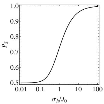
FIG. 1: Plot of $P_S$ as a function of ${\sigma }_h/J_0$ for ${\sigma }_J=0$

The expression for the return probability as a function of time, which cannot be evaluated in closed form, is

$$\begin{array}{l}{\left[P_{\uparrow \downarrow }(t)\right]}_{\alpha }=1-\frac{J_0\sqrt{\pi }}{4{\sigma }_h}{e}^{J_0^2/4{\sigma }_h^2}\mathrm{erfc}\left(\frac{J_0}{2{\sigma }_h}\right)\\ +\frac{1}{4{\sigma }_h\sqrt{\pi }}\mathrm{Re}\left[{\int }_{-\infty }^{\infty }d(\delta h)\frac{J_0^2}{J_0^2+(\delta h{)}^2}{e}^{-(\delta h{)}^2/4{\sigma }_h^2}\times e^{i\sqrt{J_0^2+(\delta h{)}^2}t}\right].\end{array}\text{\hspace{1em}(25)}$$

C. Numerical results for ${\sigma }_h=0$ and for ${\sigma }_J=0$

We now present our numerical results in the above two limits. In general, we cannot determine $T_2^{\ast }$ from an analytical formula, and thus we must extract it numerically from the return probability curve. We now describe how we do so. We attempt to find a curve of the form,

$$P_E(t)=P_S+(1-P_S)e^{-(t/T_2^{\ast }{)}^{\alpha }},\text{\hspace{1em}(26)}$$

which closely approximates the “envelope” of the return probability curve in the vicinity of the time at which the amplitude of the return probability appears to reach $1/e$ times its value at $t=0$ . We simply adjust $T_2^{\ast }$ and α until we obtain the most satisfactory fit, and then we read of $T_2^{\ast }$ We show several illustrations of this fit in Fig. 2 (the third example given is for a case in which neither ${\sigma }_h$ nor ${\sigma }_J$ are zero; we treat this general case in Sec. III D). We emphasize that we do not attempt to fit the exact “envelope” of the return probability curve for all times, but only in the vicinity of $T_2^{\ast }$ . Our typical best fit value of $\alpha$ falls in the range of 0.5–2.0 depending on the details of the parameters $(i.e.,{\sigma }_h,{\sigma }_J,J_0,etc.)$ although no significance should be attached to the precise value of $\alpha$ since all we are trying to do here is to extract an operationally meaningful value of $T_2^{\ast }$ through an accurate numerical fitting to the exact two-qubit dynamics.

We now give our results so obtained in the ${\sigma }_h=0$ and ${\sigma }_J=0$ limits. We show our results for the ${\sigma }_h=0$ limit in Fig. 3 and those for the ${\sigma }_J=0$ limit in Fig. 4.

There are two observations we make about these results. First, we have verified our approximation for $T_2^{\ast }$ for ${\sigma }_h=0$ and small ${\sigma }_J$ , but also see that the approximation appears to work very well, not just when ${\sigma }_J$ is comparable to $J_0.$ but even when it is large. The second observation is that the $T_2^{\ast }$ values that we obtain when ${\sigma }_h=0$ and ${\sigma }_J$ varies are much smaller than those that we obtain for ${\sigma }_J=0$ for comparable values of ${\sigma }_h$ . We will see later that this results in a given amount of field noise causing less of an overall loss of entanglement fidelity than an identical amount of charge noise would, despite the fact that field noise causes both a decay of the oscillations in the return probability and a shift of the steady-state return probability, while charge noise only causes a decay of oscillations.

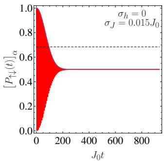
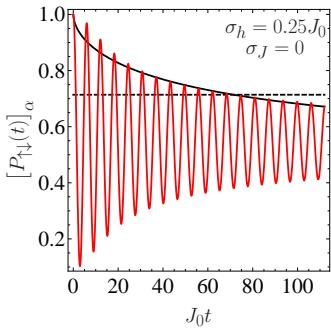
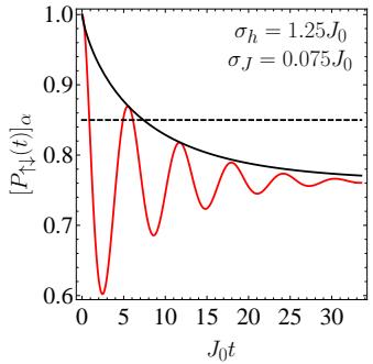
FIG. 2: Examples of our envelope-fitting procedure for ${\sigma }_h=0$ and ${\sigma }_J/J_0=0.015(\mathrm{top}$ left), ${\sigma }_h/J_0=0.25$ and ${\sigma }_J=0$ (top right), and ${\sigma }_h/J_0=1.25$ and ${\sigma }_J/J_0=0.075$ (bottom). Here, the red curve is the return probability as a function of time, the black curve is the approximation to the envelope given in $Eq.$ (26), and the dashed line is a guide showing where the amplitude of the oscillations in the return probability becomes $1/e$ times its maximum value. In these examples, the values of α and $T_2^{\ast }$ are $\alpha =2$ and $J_0{T}_2^{\ast }=94.5$ (top left), $\alpha =0.575$ and $J_0{T}_2^{\ast }=71.5$ (top right), and $\alpha =0.8$ and $J_0{T}_2^{\ast }=7.37$ (bottom).

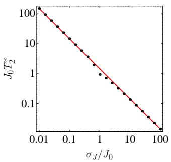
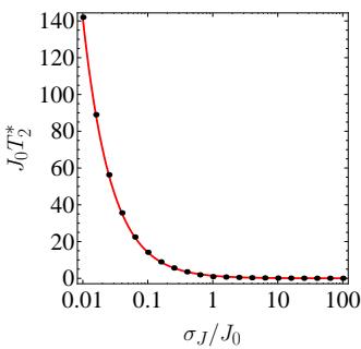
FIG. 3: Plot of $J_0{T}_2^{\ast }$ for ${\sigma }_h=0$ as a function of ${\sigma }_J/J_0$ on a log-log scale (left) and a log-linear scale $(\mathrm{right})$ . The black dots are the numerical values extracted from plots of the return probability as a function of time, while the red curves are the analytic approximation, Eq. (23), derived for small values of ${\sigma }_J/J_0$

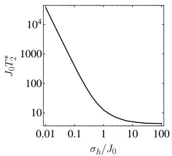
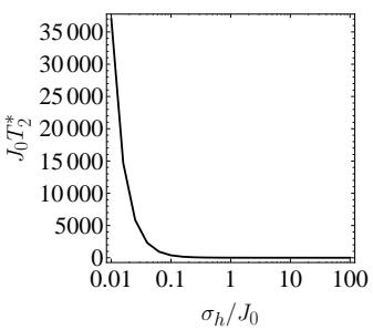
FIG. 4: Plot of $J_0{T}_2^{\ast }$ for ${\sigma }_J=0$ as a function of ${\sigma }_h/J_0$ on a log-log scale (left) and a log-linear scale (right).

D. General results

Finally, we give plots of our general results for $T_2^{\ast }$ and $P_S$ as functions of ${\sigma }_h/J_0$ and ${\sigma }_J/J_0$ We first present such plots over the region, $0\le {\sigma }_h/J_0\le 2.5$ and $0\le {\sigma }_J/J_0\le 0.15$ , in Fig. 5 since these are within the expected regime of experimental interest in GaAs and Si systems. We note that typically the charge noise is much weaker than the field noise except for isotopically pure Si where the two may be comparable in magnitude with the field noise arising simply from fluctuations in the applied magnetic field in contrast to GaAs where the main source of field noise is Overhauser nuclear field fluctuations. We find that the return probability as a function of ${\sigma }_h/J_0$ does not change noticeably if we fix ${\sigma }_J/J_0$ to a nonzero value, rather than to zero. We also see the clear trends in $T_2^{\ast }$ that our results for the ${\sigma }_h=0$ and ${\sigma }_J=0$ limits imply, namely, that it decreases if we increase either type of disorder, but increasing ${\sigma }_J/J_0$ has a quantitatively stronger efect than ${\sigma }_h/J_0$ . We indicate on these plots the strength of the disorder present in the experiments described in Ref. 15. We also present “slices” of the plot of the coherence time for constant ${\sigma }_h/J_0$ and ${\sigma }_J/J_0$ in Fig. 6.

E. “Quality factor”

We now present our results for the coherence time in an alternate form, in terms of a “quality factor”, which we may directly obtain from our results for $T_2^{\ast }$ , and which will prove useful in our discussions about entanglement fidelity below. We define this quality factor operationally as $Q:=:e^{-1/J_0{T}_2^{\ast }}$ . We first plot it over the domain of current physical interest, $0\le {\sigma }_h/J_0\le 2.5$ and

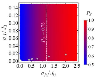
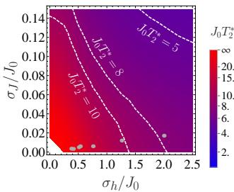
FIG. 5: (Left) Plot of the steady-state return probability $P_S$ as a function of ${\sigma }_h/J_0$ and ${\sigma }_J/J_0$ over the region, $0\le {\sigma }_h/J_0\le 2.5$ and $0\le \sigma J/J_0\le 0.15$ The dashed line indicates points at which $Ps=0.75$ . (Right) Plot of the (dimensionless) coherence time, ${\mathcal{J}}_0{\mathcal{T}}_2^{\ast }$ , over the same domain. The dashed lines indicate points at which $J_0{T}_2^{\ast }=5,$ , 8, and 10. In both plots, the gray dots represent the strength of the noise present in the experiments described in Ref. 15.

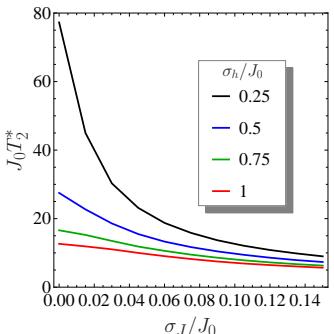
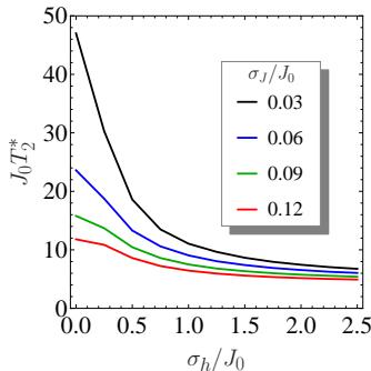
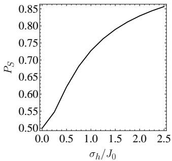
FIG. 6: (Top left) Plots of the (dimensionless) coherence time, $J_0{T}_2^{\ast }$ , as a function of ${\sigma }_J/J_0$ for several values of ${\sigma }_h/J_0$ . (Top right) Plots of the same as a function of ${\sigma }_h/J_0$ for several values of ${\sigma }_J/J_0$ . (Bottom) Plot of the return probability as a function of ${\sigma }_h/J_0$ for ${\sigma }_J=0.03J_0$ . We only present this value because the results for larger values of $\sigma J$ do not difer significantly from this curve.

$0\le {\sigma }_J/J_0\le 0.15$ , in Fig. 7; we also show “slices” of this plot for constant ${\sigma }_h/J_0$ and ${\sigma }_J/J_0$ in Fig. 8. As with our $T_2^{\ast }$ results, we also show where the experimental data of Ref. 15 fall within this region. We see that some of the experimental data already have quality factors exceeding 0.95.

Finally, we provide plots over smaller regions in Fig. 9, namely, $0\le {\sigma }_h/J_0\le 0.02$ and $0\le {\sigma }_J/J_0\le 0.02$ and $0\le {\sigma }_h/J_0\le 0.005$ and $0\le {\sigma }_J/J_0\le 0.005$ . In this case, due to the fact that the quality factors are close to

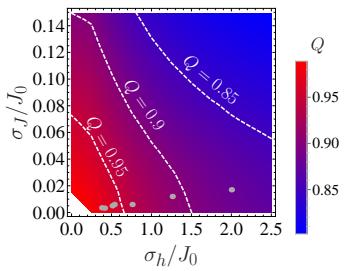
FIG. 7: Plot of the quality factor Q as a function of ${\sigma }_h/J_0$ and ${\sigma }_J/J_0$ over the domain, $0\le {\sigma }_h/J_0\le 2.5$ and $0\le \sigma J/J_0\le$ $0.15^{}$ . The dashed lines indicates points at which $Q=0.85$ $Q=0.9$ , and $Q=0.95$ . The gray dots represent the strength of the noise present in the experiments described in Ref. 15.

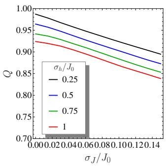
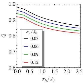
FIG. 8: (Left) Plot of the quality factor Q as a function of ${\sigma }_J/J_0$ for several values of ${\sigma }_h/J_0$ . (Right) Plot of the same as a function of ${\sigma }_h/J_0$ for several values of ${\sigma }_J/J_0$

1 (at least 0.986), we instead plot log $(1-Q)$ for visual clarity, where log is the common logarithm. The results shown in Fig. 9 provide the constraints on the noise that must be achieved in future experiments in order for the semiconductor spin quantum computing platform to approach the quantum error correction threshold.

IV. FIDELITY

We now determine the fidelity for producing the two maximally entangled states, $|M{E}_1⟩$ and $|M{E}_2⟩$ , from the unentangled state, . The fidelity $F_S$ of preparation of a state S from some initial state I is defined as the disorder-averaged probability that, upon measuring the state of the system after performing the operation O that would ideally transform I into $|S⟩$ , we will actually find it in the state $|S{⟩}^{59,60}$

$$F_S={\left[|⟨S|O|I⟩{|}^2\right]}_{\alpha }.\text{\hspace{1em}(27)}$$

We should emphasize that this definition of the fidelity is dependent on the initial state of the system and thus should not be thought of as a two-qubit entangling gate fidelity. It is more properly thought of as a state fidelity that characterizes the role of noise and decoherence in the generation of entanglement starting from a specific, unentangled initial state. However, we expect the two fidelities (our state fidelity and the entangling gate fidelity) not to be very diferent from each other; in particular, they should manifest similar qualitative dependence on the noise. Our goal is to illustrate the role of both changes in the steady-state return probability and in the intrinsic decoherence time in reducing these entanglement fidelities, assuming that we start from a maximally unentangled state. We will now apply this definition to $|M{E}_1⟩$ and $-|M{E}_2$ , which are the states that we would ideally obtain under simple time evolution by $t=\pi /2J_0$ and $t=3\pi /2J_0$ , respectively. We begin with the state, $|M{E}_1⟩$ . We find that the probability at time t for obtaining this state, starting from the initial state, , is

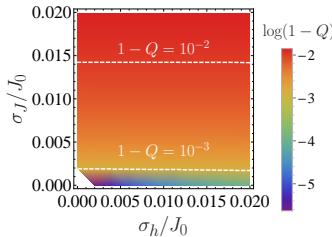
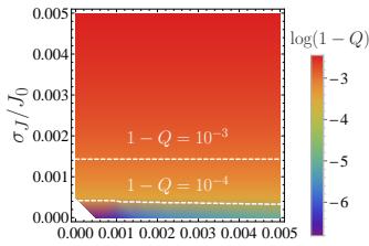
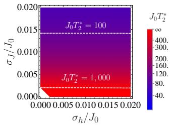
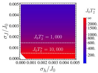
FIG. 9: Plot of the (common) logarithm of log $(1-Q)$ , where Q is the quality factor, over the regions, $0\le {\sigma }_h/J_0\le 0.02$ and $0\le \sigma J/J_0\le 0.02$ (top left) and $0\le {\sigma }_h/J_0\le 0.005$ and $0\le \sigma J/J_0\le 0.005$ (top right). We also include plots of the (dimensionless) coherence time, $J_0{T}_2^{\ast }$ , over the same regions on the bottom left and bottom right.

$$P_{M{E}_1}(t)=\frac{1}{2}+\frac{J}{2\sqrt{J^2+(\delta h{)}^2}}\sin \left[\sqrt{J^2+(\delta h{)}^2}t\right].\text{\hspace{1em}(28)}$$

The fidelity for the preparation of $|M{E}_1⟩$ is then simply the disorder average of this probability at time $t=\pi /2J_0:$

$$F_{M{E}_1}={\left[P_{M{E}_1}\left(\frac{\pi }{2J_0}\right)\right]}_{\alpha }.\text{\hspace{1em}(29)}$$

Similarly, the probability for entering the state, $|M{E}_2⟩$ ， at time t is

$$P_{M{E}_2}(t)=\frac{1}{2}-\frac{J}{2\sqrt{J^2+(\delta h{)}^2}}\sin \left[\sqrt{J^2+(\delta h{)}^2}t\right],\text{\hspace{1em}(30)}$$

and the fidelity of preparation of this state is simply the disorder average of this probability at time $t=3\pi /2J_0$

$$F_{M{E}_2}={\left[P_{M{E}_2}\left(\frac{3\pi }{2J_0}\right)\right]}_{\alpha }.\text{\hspace{1em}(31)}$$

We now evaluate these averages, first in the ${\sigma }_h=0$ and ${\sigma }_J=0$ limits, and then for general disorder strengths.

$$\mathbf{A}.{\sigma }_h=0\text{ limit }$$

We first consider the ${\sigma }_h=0$ limit. Here, we find that we can derive closed-form analytical expressions for the fidelities. We may write $F_{M{E}_1}$ as

$$\begin{array}{l}{F}_{M{E}_1}=\frac{1}{2}+\frac{1}{{\sigma }_J\sqrt{2\pi }}\frac{1}{1+\mathrm{erf}(J_0/{\sigma }_J\sqrt{2})}\\ \times \mathrm{Im}\left[{\int }_0^{\infty }dJ{e}^{-(J-J_0{)}^2/2{\sigma }_J^2+i\pi J/2J_0}\right].\end{array}\text{\hspace{1em}(32)}$$

This integral may be evaluated in terms of the error function; we obtain

$$\begin{array}{l}{F}_{M{E}_1}=\frac{1}{2}+\frac{1}{2[1+\mathrm{erf}(J_0/{\sigma }_J\sqrt{2})}\\ \times e^{-{\pi }^2{\sigma }_J^2/8J_0^2}\mathrm{Re}\left[1+\mathrm{erf}\left(\frac{J_0}{{\sigma }_J\sqrt{2}}+i\frac{\pi {\sigma }_J}{2\sqrt{2}{J}_0}\right)\right].\end{array}\text{\hspace{1em}(33)}$$

A similar calculation for $F_{M{E}_2}$ yields

$$\begin{array}{rcl}{F}_{M{E}_2}& =& \frac{1}{2}+\frac{1}{2[1+\mathrm{erf}(J_0/{\sigma }_J\sqrt{2})}\\ & \times & e^{-9{\pi }^2{\sigma }_J^2/8J_0^2}\mathrm{Re}\left[1+\mathrm{erf}\left(\frac{J_0}{{\sigma }_J\sqrt{2}}+i\frac{3\pi {\sigma }_J}{2\sqrt{2}{J}_0}\right)\right].\end{array}\text{\hspace{1em}(34)}$$

We provide plots of these fidelities in Fig. 10. We see that, while charge noise reduces the fidelity of both operations, it has a greater efect on the fidelity for producing $|M{E}_2⟩$ . This is not surprising, as this operation takes longer to execute than the one for $|M{E}_1⟩$ We also note that there is a value of ${\sigma }_J/J_0$ at which $F_{M{E}_2}$ actually goes below $\frac{1}{2}$ , then turns around and steadily increases, saturating at $\frac{1}{2}.$ , implying that the system is actually slightly more likely to go into the state, $|M{E}_1⟩$ This is likely an artifact because we truncate the distribution of exchange couplings to non-negative values only.

$$\mathbf{B}.{\sigma }_J=0\text{ limit }$$

We now consider the ${\sigma }_J=0$ limit. Unlike the ${\sigma }_h=$ 0 limit, we cannot obtain analytical expressions for the fidelities. The expressions for the fidelities are

$$\begin{array}{rl}{F}_{M{E}_1}& =\frac{1}{2}+\frac{1}{2{\sigma }_h\sqrt{\pi }}{\int }_{-\infty }^{\infty }d(\delta h)\frac{J_0}{2\sqrt{J_0^2+(\delta h{)}^2}}{e}^{-(\delta h{)}^2/4{\sigma }_h^2}\\ & \times \sin \left[\frac{\pi }{2J_0}\sqrt{J_0^2+(\delta h{)}^2}\right]\end{array}\text{\hspace{1em}(35)}$$

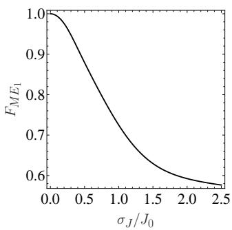
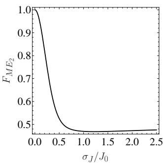
FIG. 10: Plots of $F_{M{E}_1}$ (left) and $F_{M{E}_2}(\mathrm{right})$ as a function of ${\sigma }_J/J_0$ for ${\sigma }_h=0$

and

$$\begin{array}{l}{F}_{M{E}_2}=\frac{1}{2}-\frac{1}{2{\sigma }_h\sqrt{\pi }}{\int }_{-\infty }^{\infty }d(\delta h)\frac{J_0}{2\sqrt{J_0^2+(\delta h{)}^2}}{e}^{-(\delta h{)}^2/4{\sigma }_h^2}\\ \times \sin \left[\frac{3\pi }{2J_0}\sqrt{J_0^2+(\delta h{)}^2}\right].\end{array}\text{\hspace{1em}(36)}$$

We plot these expressions in Fig. 11. We see a similar trend as before in the ${\sigma }_h=0$ limit, namely, that both fidelities are reduced, but $F_{M{E}_2}$ decreases more rapidly. We note that field noise seems to have as strong an efect on $F_{M{E}_1}$ as charge noise does, but that field noise has less of an efect on $F_{M{E}_2}$ than charge noise.

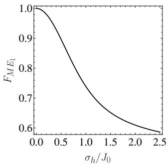
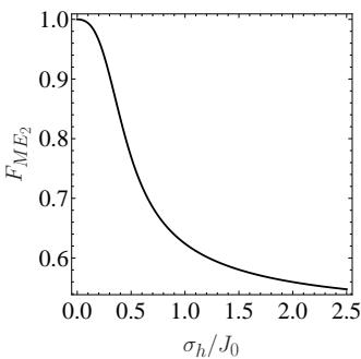
FIG. 11: Plots of $F_{M{E}_1}$ (left) and $F_{M{E}_2}$ (right) as a function of ${\sigma }_h/J_0$ for ${\sigma }_J=0$

C. General results

Finally, we present our results for arbitrary ${\sigma }_h$ and ${\sigma }_J$ We first present a plot of the fidelities $F_{M{E}_1}$ and $F_{M{E}_2}$ 2 over the region, $0<{\sigma }_h/J_0\le 2.5$ and $0<{\sigma }_J/J_0\le 0.15$ in Fig. 12, as well as “slices” of these plots for constant ${\sigma }_h/J_0$ and constant ${\sigma }_J/J_0$ in Figs. 13 and 14, respectively. We also indicate experimental values of the disorder, extracted from the data of Ref. 15. We note that fidelities for realizing the state, $|M{E}_1⟩$ , in excess of 90% have been achieved, but that those for realizing $|M{E}_2⟩$ fall short of this value. We also see that these values fall short of the threshold required in order to implement error correction codes; the surface code error correction schemes with the lowest thresholds require a fidelity of roughly 99% in all operations. Therefore, we are interested in finding the regions within which we achieve such high fidelities. We therefore present plots of both fidelities over the region, $0<{\sigma }_h/J_0\le 0.02$ and $0<{\sigma }_J/J_0\le 0.02$ , in Fig. 15, and over the region, $0<{\sigma }_h/J_0\le 0.005$ and $0<{\sigma }_J/J_0\le 0.005$ , in Fig. 16. Because of how close to 1 the fidelities are, we instead plot the common logarithm of the infidelities $I{F}_S=1-F_S$ for visual clarity. We see that, in both regions, one can already achieve a fidelity within the error correction threshold for values of ${\sigma }_h$ and ${\sigma }_J$ around $0.02J_0$ . We can also very clearly see that both types of noise have roughly the same efect on $F_{M{E}_1}$ , but that charge noise has more of an efect on $F_{M{E}_2}$ than field noise does.

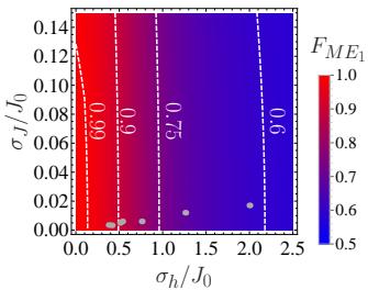
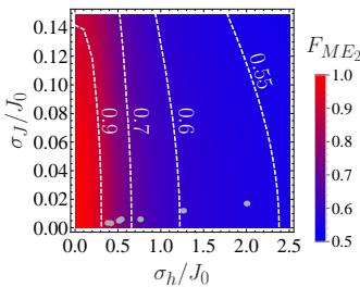
FIG. 12: Plots of $F_{M{E}_1}$ (left) and $F_{M{E}_2}$ (right) as a function of ${\sigma }_h$ and ${\sigma }_J$ over the region, $0<{\sigma }_h/J_0\le 2.5$ and $0<{\sigma }_J/J_0\le 0.15$ . We also show contours (dashed lines) over which these fidelities achieve specific values indicated on the plots. The gray dots represent the strength of the noise present in the experiments described in Ref. 15.

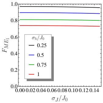
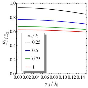
FIG. 13: Plots of the fidelities, $F_{M{E}_1}$ (left) and $F_{M{E}_2}(\mathrm{right})$ as a function of ${\sigma }_J/J_0$ for several values of ${\sigma }_h/J_0$

Overall, our results show that a given magnitude of field noise, as measured by ${\sigma }_h/J_0$ , has less of an efect on the fidelities for realizing maximally entangled states than an identical amount of charge noise, as measured by ${\sigma }_J/J_0$ . While they have identical efects on $F_{M{E}_1}$ we see that the amount of field noise needed to obtain a given efect on $F_{M{E}_2}$ is about a factor of 3 larger than the amount of charge noise needed to see the same efect. In this sense, we may claim that charge noise is more detrimental to our ability to realize a maximally entangled state than field noise. We may break down the efects caused directly by these two types of noise contributing to the decrease in fidelity as follows. Charge noise has a single efect, namely, to cause a decay of the amplitude of the oscillations in the return probability; it has no ef fect on the steady-state value of the return probability. Field noise also damps out the oscillations in the return probability, but a given amount of field noise will have less of an efect on it than the same amount of charge noise would. However, field noise has a second efect—it also increases the steady-state return probability. This, too, is harmful to the creation of a maximally-entangled state. Overall, we see that these efects result in an $F_{M{E}_1}$ that is just as adversely afected by a given amount of field noise as by the same amount of charge noise, but $F_{M{E}_2}$ is afected more strongly by charge noise than by field noise. However, we see that field noise afects $F_{M{E}_2}$ even more strongly than it does the “quality factor” Q described earlier. This shows that the damping of the oscillations of the return probability is not the only phenomenon that afects the entanglement fidelity—the fact that the return probability, and thus the initial amplitude of the return probability oscillations, difer from $\begin{array}{l}\frac{1}{2}\end{array}$ also has an efect.

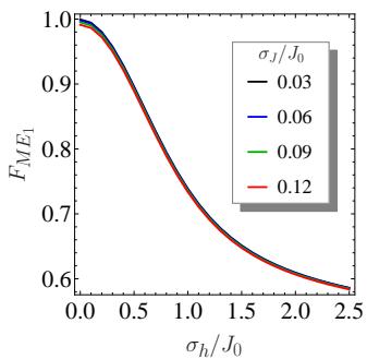
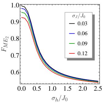
FIG. 14: Plots of the fidelities, $F_{M{E}_1}$ (left) and $F_{M{E}_2}$ (right) as a function of ${\sigma }_h/J_0$ for several values of ${\sigma }_J/J_0$

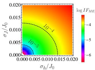
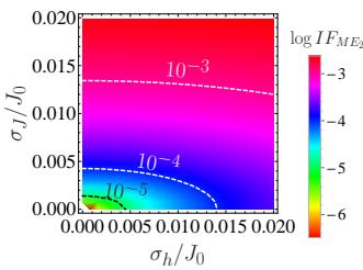
FIG. 15: Plots of the (common) logarithms of the infidelities, $I{F}_S=1-F_S$ , over the region, $0<{\sigma }_h/J_0\le 0.02$ and $0<$ ${\sigma }_J/J_0\le 0.02$ . The labels on the contours are the values of the infidelities along said contours.

We should note, however, in light of the above discussion that, in actual GaAs experimental setups, the field noise is much larger in magnitude than charge noise, as can be seen from Fig. 12. This indicates that, at least in practice, field noise is a bigger problem for entanglement in GaAs simply because it is the dominant source of noise in the system. Even in this case, we may still reduce the efect of field noise by increasing $J_0-$ note that the fidelity, like the return probability and $T_2^{\ast }$ , depends on the strength of the two types of noise only in the combinations, ${\sigma }_h/J_0$ and ${\sigma }_J/J_0$ . It turns out that, as we tune $J_0,{\sigma }_h$ remains constant, while ${\sigma }_J$ increases roughly linearly⁵⁴. This means that, while we cannot reduce the efect of charge noise by simply increasing the exchange coupling, we can reduce the efect of field noise. This is especially helpful for GaAs systems since one cannot eliminate field noise through isotopic purifica tion schemes as one can in Si. Other things being equal, however, it is obvious that Si has a great advantage over GaAs simply by virtue of its much lower field noise since Overhauser nuclear fluctuations can be almost entirely eliminated in Si, but not in GaAs. On the other hand, the advantage of having much weaker field noise in Si would be seriously compromised if the charge noise in Si turns out to be stronger than in GaAs.

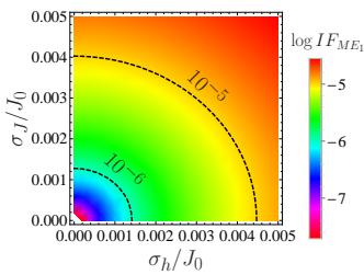
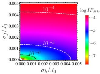
FIG. 16: Plots of the (common) logarithms of the infidelities, $I{F}_S=1-F_S$ , over the region, $0<{\sigma }_h/J_0\le 0.005$ and $0<$ ${\sigma }_J/J_0\le 0.005$ . The labels on the contours are the values of the infidelities along said contours.

V. DISCUSSION

We have determined the intrinsic coherence time, $T_2^{\ast }$ the steady-state return probability, $P_S,$ , and the fidelities $F_{M{E}_1}$ and $F_{M{E}_2}$ for producing the maximally entangled states $|M{E}_1⟩$ and ME₂ , respectively, starting from the unentangled state, , for a system of two electron spins coupled via the Heisenberg exchange coupling with both magnetic field and charge noise as a function of the strength of both types of noise. We employed the quasistatic bath approximation, taking the distributions for both types of noise to be Gaussian; in the case of charge noise, we truncated the distribution so that the exchange coupling is always positive. These results are of direct and immediate relevance to current quantum computing experiments on coupled electron spins in quantum dots since we have focused on standard experimental observables (return probability) and used realistic noise models. In fact, we indicate the values of the disorder that have recently been estimated experimentally in our presented results¹⁵. The main goal of our work is to calculate the fidelity of operations that maximally entangle two electron spins, starting from an unentangled state. This is an important problem, as universal quantum computation requires the ability to perform at least one such two-qubit operation, along with arbitrary single-qubit rotations.

We find that, while both types of noise suppress $T_2^{\ast }$ electronic noise has a far greater efect, indicating that charge noise is much more efective at causing decoherence in the system than field noise. We also calculate the steady-state return probability and show that only field noise has any significant efect on it. While the fact that charge noise lowers $T_2^{\ast }$ more than field noise would at first seem to indicate that it is much more harmful to our ability to entangle the electronic spins, the situation is more subtle in the presence of both types of noise. Because charge noise does not change the steadystate return probability, our “na¨ıve” entangling operation still closely approximates the ideal SWAP entangling operation as long as it is performed over a time scale much smaller than $T_2^{\ast }$ . This is not the case with field noise, however: any amount of field noise will change the steady-state return probability, and thus our “na¨ıve” operation will deviate from the ideal $\sqrt{\mathrm{SWAP}}$ entangling operation regardless of how quickly it is performed. We thus expect that field noise is more harmful to perform ing such an operation than our results for $T_2^{\ast }$ would suggest, and this is in fact borne out in our results for the entanglement fidelities. We find that $F_{M{E}_1}$ is just as greatly reduced by a given magnitude of field noise as by an equal amount of charge noise. On the other hand, $F_{M{E}_2}$ is not afected as much by field noise as it is by charge noise, but it is still reduced more than the “qual ity factor” $\dot{Q}=e^{-1/J_0{T}_2^{\ast }}$ is. This fact helps to illustrate the efect of the steady-state return probability shift on the fidelity. One must, however, take into account the fact that field and charge noise are typically not of com parable magnitudes in semiconductors, and thus, their actual harmful efects on two-qubit operations would depend strongly on their actual magnitudes. This is why we have presented results in this work covering wide pa rameter regimes for both field and charge noise strengths.

Our results imply that a given amount of charge noise overall has a more detrimental efect on entanglement fidelity than an equal amount of field noise; while both types of noise afect the fidelity for producing $|M{E}_1⟩$ equally, charge noise has more of an efect on that for producing $|M{E}_2⟩$ than field noise does. We see, however, that, at least in GaAs, field noise is much stronger than charge noise, and thus is a bigger problem in this material. Such noise, however, can be made much smaller in Si than in $\mathrm{GaAs},$ since isotopic purification can greatly reduce the presence of magnetic isotopes of Si ${(}^{29}\mathrm{Si}$ , to be exact), while no such reduction is possible in GaAs because the only stable isotopes of Ga and As have nonzero spin. The same concerns about unavoidable field noise in GaAs arise in P-doped Si as well owing to the fact that the only stable isotope of $\mathrm{P},{}^{31}\mathrm{P}.$ has a non-zero spin; however, the field noise will not be as great as in

GaAs since not all of the nuclei present in the sample are magnetic. There is, however, another way to reduce the efects of field noise that works for both materials. We can take advantage of the fact that ${\sigma }_h$ essentially remains constant as one changes the average exchange coupling $J_0,$ while ${\sigma }_J$ is roughly linear⁵⁴ in $J_0$ . This means that, since the fidelities and the return probability depend only on ${\sigma }_h/J_0$ and ${\sigma }_J/J_0$ , one can reduce the efects of field noise simply by increasing $J_0.$ . In fact, as can be seen from the experimental points indicated in Fig. 12, it is possible to achieve fidelities in excess of 90% for producing the state $|M{E}_1⟩$ or close to 90% for producing $|M{E}_2⟩$ in current GaAs-based experimental setups by doing this. Recent experimental work²⁸ suggests that a similar approach can be used to suppress charge noise by creating a large magnetic field gradient across the double quantum dot, provided Bayesian estimation or dynamical decoupling are used simultaneously to mitigate field noise. Our findings indicate that if both ${\sigma }_h/J_0$ and ${\sigma }_J/J_0$ are reduced down to the 1% level, then entanglement fidelities at or beyond surface code thresholds of 99% can be achieved.

Our work also implies that Si systems in the end are far superior to GaAs in terms of achieving ideal two-qubit gate operations by virtue of the fact that in Si the field

¹ F. Zwanenburg, A. S. Dzurak, A. Morello, M. Y. Simmons, L. C. L. Hollenberg, G. Klimeck, S. Rogge, S. N. Coppersmith, and M. A. Eriksson, Rev. Mod. Phys. 85, 961 (2013).

² D. Loss and D. P. DiVincenzo, Phys. Rev. A 57, 120 (1998).

³ J. Pla, K. Y. Tan, J. P. Dehollain, W. H. Lim, J. J. L. Morton, D. N. Jamieson, A. S. Dzurak, and A. Morello, Nature (London) 489, 541 (2012).

J. Pla, K. Y. Tan, J. P. Dehollain, W. H. Lim, J. J. L. Morton, F. A. Zwanenburg, D. N. Jamieson, A. S. Dzurak and A. Morello, Nature (London) 496, 334 (2013).

5 M. Veldhorst, J. C. C. Hwang, C. H. Yang, A. W. Leenstra, B. de Ronde, J. P. Dehollain, J. T. Muhonen, F. E. Hudson, K. M. Itoh, A. Morello, and A. S. Dzurak, Nature Nano. 9, 981 (2014).

⁶ F. R. Braakman, P. Barthelemy, C. Reichl, W. Wegscheider, and L. M. K. Vandersypen, Nature Nano. 8, 432-437 (2013).

⁷ T. Otsuka, T. Nakajima, M. R. Delbecq, S. Amaha, J. Yoneda, K. Takeda, G. Allison, T. Ito, R. Sugawara, A. Noiri, A. Ludwig, A. D. Wieck, and S. Tarucha, Sci. Rep. 6, 31820 (2016).

⁸ T. Ito, T. Otsuka, S. Amaha, M. R. Delbecq, T. Nakajima, J. Yoneda, K. Takeda, G. Allison, A. Noiri, K. Kawasaki, and S. Tarucha, arXiv:1604.04426.

⁹ J. Levy, Phys. Rev. Lett. 89, 147902 (2002).

¹⁰ J. R. Petta, A. C. Johnson, J. M. Taylor, E. A. Laird, A. Yacoby, M. D. Lukin, C. M. Marcus, M. P. Hanson, A. C. Gossard, Science 309, 2180 (2005).

¹¹ S. Foletti, H. Bluhm, D. Mahal, V. Umansky, and A. Yacoby, Nature Phys. 5, 903 (2009).

noise can, in principle, be reduced to arbitrarily small values by eliminating background nuclear spin fluctuations. Charge noise, on the other hand, is likely to be similar in both systems. Therefore, Si obviously has a great advantage over GaAs in terms of noise. This is not to say that Si has a clear advantage over GaAs; there are challenges associated with Si as a material platform as well. For one, the charge carriers in Si have a much higher efective mass than in GaAs. This means that one is forced to fabricate much smaller dots in order to confine individual electrons. Another issue is valley degeneracy of energy levels, which complicates the task of isolating two nondegenerate levels to use as qubit states. Valley efects relevant to Si quantum dots have been studied to some extent in the literature^62,63. Our detailed numerical results presented in this paper provide a quantitative guide on how much both types of noise must be suppressed in experimental systems for achieving the fidelities above 99% that are necessary for further progress in the field.

Acknowledgments

This work is supported by LPS-MPO-CMTC.

12 B. Maune, M. G. Borselli, B. Huang, T. D. Ladd, P. W. Deelman, K. S. Holabird, A. A. Kiselev, I. Alvarado-Rodriguez, R. S. Ross, A. E. Schmitz, M. Sokolich, C. A. Watson, M. F. Gyure, and A. T. Hunter, Nature (London) 481, 344 (2012).

¹³ M. Shulman, S. P. Harvey, J. M. Nichol, S. D. Bartlett, A. C. Doherty, V. Umansky, and A. Yacoby, Nature Commun. 5, 5156 (2014).

¹⁴ O. E. Dial, M. D. Shulman, S. P. Harvey, H. Bluhm, V. Umansky, and A. Yacoby, Phys. Rev. Lett. 110, 146804 (2013).

15 F. Martins, F. K. Malinowski, P. D. Nissen, E. Barnes, S. Fallahi, G. C. Gardner, M. J. Manfra, C. M. Marcus, and F. Kuemmeth, Phys. Rev. Lett. 116, 116801 (2016).

¹⁶ D. P. DiVincenzo, D. Bacon, J. Kempe, G. Burkard, and K. B. Whaley, Nature (London) 408, 339 (2000).

17 J. Medford, J. Beil, J. M. Taylor, S. D. Bartlett, A. C. Doherty, E. I. Rashba, D. P. DiVincenzo, H. Lu, A. C. Gossard, and C. M. Marcus, Nature Nano. 8, 654 (2013).

18 J. Medford, J. Beil, J. M. Taylor, E. I. Rashba, H. Lu, A. C. Gossard, and C. M. Marcus, Phys. Rev. Lett. 111, 050501 (2013).

19 K. Eng, T. D. Ladd, A. Smith, M. G. Borselli, A. A. Kiselev, B. H. Fong, K. S. Holabird, T. M. Hazard, B. Huang, P. W. Deelman, I. Milosavljevic, A. E. Schmitz, R. S. Ross, M. F. Gyure, and A. T. Hunter, Sci. Adv. 1, e150021 (2015).

²⁰ Y.-P. Shim and C. Tahan, Phys. Rev. B 93, 121410 (2016).

²¹ Z. Shi, C. B. Simmons, J. R. Prance, J. K. Gamble, T. S. Koh, Y.P. Shim, X. Hu, D. E. Savage, M. G. Lagally, M. A. Eriksson, M. Friesen, and S. N. Coppersmith, Phys. Rev. Lett. 108, 140503 (2012).

22 D. Kim, Z. Shi, C. B. Simmons, D. R. Ward, J. R. Prance, T. S. Koh, J. K. Gamble, D. E. Savage, M. G. Lagally, M. Friesen, S. N. Coppersmith, and M. A. Eriksson, Nature (London) 511, 70 (2014).

²³ D. Kim, D. R. Ward, C. B. Simmons, D. E. Savage, M. G. Lagally, M. Friesen, S. N. Coppersmith, and M. A. Eriksson, npj Quant. Inf. 1, 15004 (2015).

²⁴ I. van Weperen, B. D. Armstrong, E. A. Laird, J. Medford, C. M. Marcus, M. P. Hanson, and A. C. Gossard, Phys. Rev. Lett. 107, 030506 (2011).

25 M. Veldhorst, C. H. Yang, J. C. C. Hwang, W. Huang, J. P. Dehollain, J. T. Muhonen, S. Simmons, A. Laucht, F. E. Hudson, K. M. Itoh, A. Morello, and A. S. Dzurak, Nature 526, 410 (2016).

²⁶ K. Nowack, M. Shafiei, M. Laforest, G. E. D. K. Prawiroatmodjo, L. R. Schreiber, C. Reichl, W. Wegscheider, and L. M. K. Vandersypen, Science 333, 1269 (2011).

²⁷ M. Shulman, O. E. Dial, S. P. Harvey, H. Bluhm, V. Umansky, and A. Yacoby, Science 336, 202 (2012).

28 J. M. Nichol, L. A. Orona, S. P. Harvey, S. Fallahi, G. C. Gardner, M. J. Manfra, and A. Yacoby, arXiv:1608.04258.

29 A. G. Fowler, M. Mariantoni, J. M. Martinis, and A. N. Cleland, Phys. Rev. A 86, 032324 (2012).

³⁰ R. de Sousa and S. Das Sarma, Phys. Rev. B 67, 033301 (2003).

³¹ X. Hu and S. Das Sarma, Phys. Rev. Lett. 96, 100501 (2006).

³² L. Viola and S. Lloyd, Phys. Rev. A 58, 2733 (1998).

³³ L. Cywinski, R. M. Lutchyn, C. P. Nave, and S. Das Sarma, Phys. Rev. B 77, 174509 (2008).

³⁴ H. Bluhm, S. Foletti, D. Mahalu, V. Umansky, and A. Yacoby, Phys. Rev. Lett. 105, 216803 (2010).

35 F. K. Malinowski, F. Martins, P. D. Nissen, E. Barnes, L. Cywi´nski, M. S. Rudner, S. Fallahi, G. C. Gardner, M. J. Manfra, C. M. Marcus, F. Kuemmeth, Nat. Nanotechnol. 12, 16 (2017).

³⁶ A. Sergeevich, A. Chandran, J. Combes, S. D. Bartlett, and H. M. Wiseman, Phys. Rev. A 84 052315 (2011).

³⁷ W. M. Witzel, M. S. Carroll, A. Morello, L. Cywi´nski, and S. Das Sarma, Phys. Rev. Lett. 105, 187602 (2010).

³⁸ X. Wang, L. S. Bishop, J. P. Kestner, E. Barnes, K. Sun, and S. Das Sarma, Nature Commun. 3, 997 (2012).

³⁹ J. P. Kestner, X. Wang, L. S. Bishop, E. Barnes, and S. Das Sarma, Phys. Rev. Lett. 110, 140502 (2013).

⁴⁰ X. Wang, L. S. Bishop, E. Barnes, J. P. Kestner, and S.

Das Sarma, Phys. Rev. A 89, 022310 (2014).

⁴¹ K. Khodjasteh, H. Bluhm, and L. Viola, Phys. Rev. A 86, 042329 (2012).

⁴² E. Barnes, X. Wang, and S. Das Sarma, Sci. Rep. 5, 12685 (2015).

⁴³ G. S. Uhrig, Phys. Rev. Lett. 98, 100504 (2007).

⁴⁴ W. M. Witzel and S. Das Sarma, Phys. Rev. Lett. 98, 077601 (2007).

45 B. Lee, W. M. Witzel, and S. Das Sarma, Phys. Rev. Lett. 100, 160505 (2008).

⁴⁶ W. Yao, R.B. Liu, and L. J. Sham, Phys. Rev. Lett. 98, 077602 (2007).

⁴⁷ T. Yu and J. H. Eberly, Phys. Rev. B 68, 165322 (2003).

⁴⁸ K. Ann and G. Jaeger, Phys. Rev. B 75 115307 (2007).

49 A. De, A. Lang, D. Zhou, and R. Joynt, Phys. Rev. A 83, 042331 (2011).

⁵⁰ I. Bragar, and L. Cywi´nski, Phys. Rev. B 91, 155310 (2015).

⁵¹ P. Sza´nkowski, M. Trippenbach, L. Cywi´nski, and Y. B. Band, Quantum Info. Process. 14, 3367 (2015).

⁵² W. A. Coish and D. Loss, Phys. Rev. B 72, 125337 (2005).

⁵³ D. Klauser, W. A. Coish, and D. Loss, Phys. Rev. B 73, 205302 (2006).

⁵⁴ E. Barnes, M. S. Rudner, F. Martins, F. K. Malinowski, C. M. Marcus, and F. Kuemmeth, Phys. Rev. B 93, 121407R (2016).

⁵⁵ S. Das Sarma, R. E. Throckmorton, and Y.-L. Wu, Phys. Rev. B 94, 045435 (2016).

⁵⁶ L. Cywi´nski, Acta Phys. Pol. 119, 576 (2011).

⁵⁷ I. Neder, M. S. Rudner, H. Bluhm, S. Foletti, B. I. Halperin, and A. Yacoby, Phys. Rev. B 84, 035441 (2011).

58 J. Medford, L. Cywi´nski, C. Barthel, C. M. Marcus, M. P. Hanson, and A. C. Gossard, Phys. Rev. Lett. 108, 086802 (2012).

59 M. A. Nielsen and I. L. Chuang, Quantum Computation and Quantum Information (Cambridge University Press, Cambridge, 2000).

⁶⁰ E. Magesan, J. M. Gambetta, and J. Emerson, Phys. Rev. A 85, 042311 (2012).

⁶¹ T. D. Ladd, Phys. Rev. B 86, 125408 (2012)

⁶² X. Hao, R. Ruskov, M. Xiao, C. Tahan, and H.-W. Jiang, Nature Commun. 5, 3860 (2014).

⁶³ Y. Song and S. Das Sarma, Appl. Phys. Lett. 109, 253113 (2016).