A Superconducting Persistent Current Qubit

Orlando et al., doi:cond-mat/9908283 的机器可读全文页。

文献信息

Orlando et al., doi:cond-mat/9908283，“A Superconducting Persistent Current Qubit”. DOI:cond-mat/9908283 原文为 arXiv 预印本版本的机器可读转换，公式与图注以原文为准；本页仅作站内索引与全文查阅，引用请以正式出版物为准。

全文

A Superconducting Persistent Current Qubit

T. P. Orlando^a, J. E. Mooij^a,b, Lin Tian^c, Caspar H. van der Wal^b, L. Levitov^c, Seth Lloyd^d, J. J. Mazo^a,e

^aDept. of Electrical Engineering & Computer Science, M.I.T., Cambridge, MA, 02139, USA

^bDept. of Applied Physics, Delft University of Technology, P.O.Box 5046, 2628 CJ Delft, The Netherlands

^cDept. of Physics, M.I.T., Cambridge, MA, 02139, USA

^dDept. of Mechanical Engineering, M.I.T., Cambridge, MA, 02143, USA ^e Departamento de F´ısica de la Materia Condensada and ICMA, CSIC-Universidad de Zaragoza, E-50009 Zaragoza, Spain (November 26, 2024)

We present the design of a superconducting qubit that has circulating currents of opposite sign as its two states. The circuit consists of three nano-scale aluminum Josephson junctions connected in a superconducting loop and controlled by magnetic fields. The advantages of this qubit are that it can be made insensitive to background charges in the substrate, the flux in the two states can be detected with a SQUID, and the states can be manipulated with magnetic fields. Coupled systems of qubits are also discussed as well as sources of decoherence.

I. INTRODUCTION

Quantum computers are devices that store information on quantum variables such as spins, photons, and atoms, and that process that information by making those variables interact in a way that preserves quantum coherence [1–5]. Typically, these variables consist of two-state quantum systems called quantum bits or ‘qubits’ [6]. To perform a quantum computation, one must be able to prepare qubits in a desired initial state, coherently manipulate superpositions of a qubit’s two states, couple qubits together, measure their state, and keep them relatively free from interactions that induce noise and decoherence [1–4,7,8]. Qubits have been physically implemented in a variety of systems, including cavity quantum electrodynamics [9], ion traps [10], and nuclear spins [11,12]. Essentially any two-state quantum system that can be addressed, controlled, measured, coupled to its neighbors and decoupled from the environment, is potentially useful for quantum computation and quantum communications [13,14]. Electrical systems which can be produced by modern lithography, such as nano-scaled quantum dots and tunnel junctions, are attractive candidates for constructing qubits: a wide variety of potential designs for qubits and their couplings are available, and the qubits are easily scaled to large arrays which can be integrated in electronic circuits [3,15]. For this reason mesoscopic superconducting circuits of ultra-small Josephson junctions have been proposed as qubits [16–20] and we detail one such circuit in this paper.

Compared with the photonic, atomic, and nuclear qubits already constructed, solid state proposals based on lithography such as the one described here have two considerable disadvantages and one considerable advantage. The first disadvantage is noise and decoherence [3,7,8]: the solid state environment has a higher density of states and is typically more strongly coupled to the degrees of freedom that make up the qubit than is the environment for photons in cavities, ions in ion traps, and nuclear spins in a molecule or crystal. Extra care must be taken in solid state to decouple the qubit from all sources of noise and decoherence in its environment. The second disadvantage is manufacturing variability [8]: each ion in an ion trap is identical by nature, while each lithographed Josephson junction in an integrated circuit will have slightly diferent properties. Solid state designs must either be insensitive to variations induced by the manufacturing process, or must include a calibration step in which the parameters of diferent subcircuits are measured and compensated for [15].

The advantage of solid state lithographed circuits is their flexibility: the layout of the circuit of Josephson junctions or quantum dots is determined by the designer, and its parameters can be adjusted continuously over a wide range. As the results presented in this paper demonstrate, this flexibility allows the design of circuits in which the variables that register the qubits are only weakly coupled to their environment. In addition, the flexibility in circuit layout allows many possible options for coupling qubits together, and for calibrating and adjusting the qubits’ parameters. That is, the advantage of flexibility in design can compensate for the disadvantages of decoherence and manufacturing variability.

The flexibility in design aforded by lithography conveys a further advantage to constructing quantum computers. As noted above, a qubit has to accomplish at least five functions: it has to be addressed, controlled, measured, coupled to its neighbors and decoupled from the environment. One of the axioms of design, is that the number of parameters that characterize a system’s design should be at least as great as the number of parameters that characterize the system’s function [21]. The problem of having too few design parameters available is particularly acute in the design of quantum computers and qubits : a quantum computer is a device in which essentially every physical degree of freedom is used to register information and to perform the computation. Degrees of freedom that are not used to compute are sources of noise and must be isolated from the computing degrees of freedom. Designs for quantum computers are accordingly more constrained by fundamental physics than are designs for conventional computers: if one is storing information on a cesium atom, then the “design parameters” of the cesium atom —its energy levels, decoherence times, interaction strengths, etc. —are fixed by nature once and for all. In the lithographed Josephson junction circuits proposed here, by contrast, it is possible to make qubits that have a variety of diferent design parameters, each of which can be adjusted to optimize diferent functions.

II. JOSEPHSON-JUNCTION QUBITS

The superconducting Josephson tunnel junction is described by a critical current $I_o$ and a capacitance C. (We will assume that the resistive channel of the junction is negligibly small.) For superconducting circuits the geometrical loop inductance $L_s$ is also important if $\Lambda =L_J/L_s<1$ , where $L_J={\Phi }_o/2\pi I_c$ is the inductance associated with a Josephson junction in the loop. Here ${\Phi }_o=h/2e$ is the superconducting flux quantum. Josephson circuits can be divided into two general categories. Circuits of the first type have $\Lambda \gg 1$ so that the induced flux in the loop is not important. These circuits are typically made of aluminum, and the mesoscopic nature of their electronic transport has been studied in nanoscaled circuits. Circuits of the second type have $\Lambda \ll 1$ and induced flux caused by circulating currents is important. These circuits are typically made of niobium, and the macroscopic nature of the tunneling of flux has been studied in small-scaled circuits.

The prospects of using superconducting circuits of the first type as qubits is encouraging because extensive experimental and theoretical work has already been done on mesoscopic superconducting circuits. (For a review of this work see Chapter 7 in [22] and in Ref. [23].) In circuits of the first type $(\Lambda \gg 1)$ , two energy scales determine the quantum mechanical behavior: The Josephson coupling energy, $E_J=I_o{\Phi }_o/2\pi$ 2 and the coulomb energy for single charges, $E_c=e^2/2C$ . The energies can be determined by the phases of the Cooper pair wave function of the nodes (islands) and the number of excess Cooper pairs on each node. The phase and the number can be expressed as quantum mechanical conjugate variables [24].

In the “superconducting” limit $E_J>E_c$ , the phase is well defined and the charge fluctuates. In the “charging” limit, the charges on the nodes are well defined and the phase fluctuates strongly. When $E_J$ and $E_c$ are within a few orders of magnitude of each other, the eigen states must be considered as quantum mechanical superpositions of either charge states or phase states. Such superposition states are important in designing qubits. Experimental studies have been performed by several groups with aluminum tunnel junctions with dimensions below 100 nm [22,23]. Superposition of charge states in circuits in the charging regime have been demonstrated [25–27] and are in quantitative agreement with theory [28,29]. The Heisenberg uncertainty principle has been demonstrated when $E_J\approx E_c:[30,26]$ . When $E_J>E_c$ topological excitations known as vortices exists and quantum mechanical interference of these quantities has been observed [31]. Unfortunately circuits of the first type in the charging regime are sensitive to fluctuating of-set charges that are present in the substrate [32,33]. These random of-set charges make dificult the design of a controllable array of quantum circuits and introduce a strong source of decoherence.

In circuits of the second type $(\Lambda \ll 1)$ , the quantum variables can be related to the flux in the loops and their time derivatives. For a superconducting loop with a single Josephson junction, known as an rf SQUID, thermal activation of macroscopic quantum states [34] has been observed as well as macroscopic quantum tunneling between states and the discrete nature of the quantum states [35]. One of the advantages of these rf SQUID systems is that the two states have circulating currents of opposite sign and, hence, produce a readily measurable flux of opposite signs. To date no superposition of states have been demonstrated in the niobium circuits, although the improving quality of the niobium tunnel junctions may allow such a demonstration [36,37].

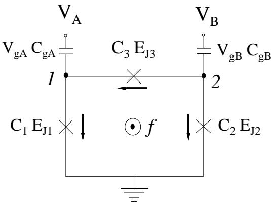
FIG. 1. The three-junction qubit. Josephson junctions 1 and 2 both have Josephson energies $E_J$ and capacitance C and Josephson junction 3 has a Josephson energy and capacitance α times larger. The nodes 1 and 2 represent the superconducting islands (nodes) which are coupled by gate capacitors $C_g=\gamma C$ to gate voltages $V_A$ and $V_B$ . The arrows define the direction of the currents. The flux is taken out of the page.

The goal of this paper is to design a qubit using circuits of the first type with aluminum, yet to have states (like in circuits of the second type) that are circulating currents of opposite sign. These circulating current states create a magnetic flux of about $10^{-3}{\Phi }_o$ and we refer to these as “persistent current (PC) states.” These states obey all five functional requirements for a quantum bit: (1) The superconducting circuit is at suficiently a low temperature that the the PC states can be made insensitive to background charges and effectively decoupled from their electrostatic environment. The magnetic coupling to the PC states and the environment can also be made suficiently weak.

III. THE CIRCUIT

The circuit of the qubit is shown in Fig. 1. Each junction is marked by an ${}^{66}{\mathrm{x}}^{55}$ and is modeled [22,38] by a parallel combination of an ideal Josephson junction and a capacitor $C_i.$ The parallel resistive channel is assumed negligible. The ideal Josephson junction has a current-phase relation, $I_i=I_o$ sin ${\phi }_i$ where ${\phi }_i$ is the gauge-invariant phase of junction i.

For the calculation of the energy the inductance of the loop is considered negligible $\Lambda \gg 1$ so that the total flux is the external flux. In this case, fluxoid quantization around the loop containing the junctions, gives ${\phi }_1-{\phi }_2+{\phi }_3=-2\pi f$ . Here $f$ is the magnetic frustration and is the amount of external magnetic flux in the loop in units of the flux quantum ${\Phi }_o$

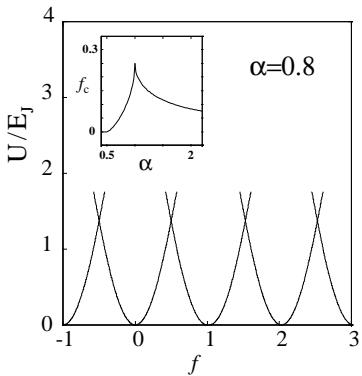
FIG. 2. $U/E_J$ vs. $f$ for $\alpha =0.8$ and for minimum energy phase configuration. The energy is periodic with period $f=1$ and is symmetric about $f=1/2$ . Near $f=1/2,$ , there is a region $[1/2-f_c,1/2+f_c]$ where there are two stable solutions. The inset plots $f_c$ as a function of $\alpha$ .

The Josephson energy due to each junction is $E_{Jn}(1-$ $\cos {\phi }_n)$ The total Josephson energy $U$ is then $\begin{array}{rl}U& =\end{array}$ $\begin{array}{r}{\sum }_i{E}_{Ji}(1-\cos {\phi }_i)\end{array}$ . Combined with the flux quantization con-Pdition the Josephson energy is [39]

$$\frac{U}{E_J}=2+\alpha -\cos {\phi }_1-\cos {\phi }_2-\alpha \cos (2\pi f+{\phi }_1-{\phi }_2).\text{\hspace{1em}(1)}$$

The important feature of this Josephson energy is that it is a function of two phases [40]. For a range of magnetic frustration $f,$ these two phases, ϕ₁ and ${\phi }_2$ , permit two stable configurations which correspond to dc currents flowing in opposite directions. We illustrate this in Fig. 2, where we plot the energy of the minimum of the system as a function of $f$ for $\alpha =0.8$ . The energy is periodic with period $f=1$ and is symmetric about $f=1/2$ . Near $f=1/2$ , there is a region $[1/2-f_c,1/2+f_c]$ where there are two stable solutions. The inset plots $f_c$ as a function of $\alpha$ . These two solutions have circulating currents of opposite direction and are degenerate at $f=1/2$ . The calculation of the energy for the stable solutions and $f_c$ is given in Appendix A.

The main feature of the qubit that is proposed in this paper is to use these two states of opposite current as the two states of the qubit. By adding the charging energy (the capacitive energy) of the junctions and considering the circuit quantum mechanically, we can adjust the parameters of the circuit so that the two lowest states of the system near $f=1/2$ will correspond to these two classical states of opposite circulating currents. Moreover, we will show that these two states can be made insensitive to the gate voltages and the random ofset charges. The quantum mechanics of the circuit will be considered in detail in the next section.

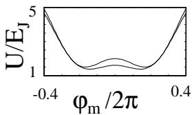
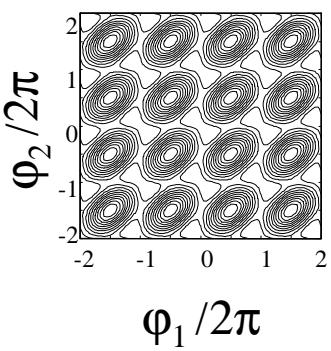
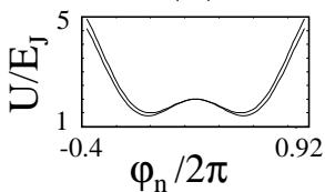
The stable classical solutions correspond to energy minima in $U({\phi }_1,{\phi }_2)$ ). Let’s consider the case of $f=1/2$ . For $\alpha \le 1/2$ $U$ has only one minimum at ${\phi }_1={\phi }_2=0$ mod 2π. Above the critical value of $\alpha =1/2$ , this minimum bifurcates into two degenerate minima at ${\phi }_1=-{\phi }_2=\pm {\phi }^{\ast }$ mod 2π where cos ${\phi }^{\ast }=1/2\alpha$ . The minima form a two-dimensional pattern with the two minima at $({\phi }^{\ast },-{\phi }^{\ast })$ and $(-{\phi }^{\ast },{\phi }^{\ast })$ repeated in a two-dimensional square lattice. This pattern can be seen in Fig. 3 which is a contour plot of the Josephson energy as a function of the phase variables for $\alpha =0.8$ The nested nearly circular contours mark the maxima in the potential. The figure-eight shaped contour encloses two minima. Fig. 3b shows the potential along ${\phi }_m,$ the phase between the two minimum in a unit cell; that is, along the line ${\phi }_2=-{\phi }_1$ . The upper curve is for $\alpha =1.0$ and the lower for $\alpha =0.8$ . Fig. 3c shows the potential vs ${\phi }_n.$ which connects one minimum (say at $(-{\phi }^{\ast },{\phi }^{\ast }))$ ) to its next nearest neighbor (at $({\phi }^{\ast },2\pi -{\phi }^{\ast }))$ For $\alpha =0.8$ the energy barrier between the two minima is much lower than the energy barrier from the minimum in one unit cell to the neighboring unit cell. For $\alpha =1.0$ the energy barrier from unit cell to unit cell is nearly the same as the barrier within the unit cell. The ability to manipulate the potential landscape by changing α will be important in designing the qubit.

(a)

(b)

(c)
FIG. 3. (a) A contour plot of the Josephson energy (potential energy) $U\left({\phi }_1,{\phi }_2\right)$ for $f=1/2$ for $\alpha =0.8$ . The nested nearly circular shapes mark the maxima in the potential, and the figure-eight shaped contours enclose two minima. (b) A plot of the potential vs. ${\phi }_m,$ the phase along the direction between these two minimum in the same unit cell, (c) A plot of the potential vs. ${\phi }_n,$ the phase along direction from one minima to its next nearest neighbor. Note that the barrier is a saddle point. The upper curve in each figure is for $\alpha =1.0$ and the lower for $\alpha =0.8$

We now consider the electric energy $T$ stored in the five capacitors in the circuit. Each capacitor $C_j$ has a voltage across it of $V_j$ so that

$$T=\frac{1}{2}\sum _j{C}_j{V}_j^2-Q_{gA}{V}_A-Q_{gB}{V}_B.\text{\hspace{1em}(2)}$$

Here $j=1,2,3$ and $gA$ and $gB$ . The last two terms subtract the work done by the voltage source to give the available electric (free) energy [41]. The voltage across each Joseph son junction is given by the Josephson voltage-phase relation $V_n=({\Phi }_o/2\pi ){\dot{\phi }}_n$ , where the over-dot indicates a partial time derivative. The ground in the circuit labels the zero of potential and is a virtual ground.

The voltage across the gate capacitor $gA$ is $V_{gA}=V_A-V_1$ and similarly for $V_{gB}=V_B-V_2$ . The electric energy can then be written in terms of the time derivatives of the phases as

$$T=\frac{1}{2}{\left(\frac{{\Phi }_0}{2\pi }\right)}^2{\vec{\phi }}^T\cdot \mathbf{C}\cdot \vec{\phi }.\text{\hspace{1em}(3)}$$

The constant term $-\frac{1}{2}{\vec{V}}_g^T\cdot {\mathbf{C}}_g\cdot {\vec{V}}_g$ has been neglected and

$$\vec{\phi }=\left(\genfrac{}{}{0ex}{}{{\dot{\phi }}_1}{{\dot{\phi }}_2}\right)\mathbf{C}=C\left(\begin{array}{cc}1+\alpha +\gamma & -\alpha \\ -\alpha & 1+\alpha +\gamma \end{array}\right)\text{\hspace{1em}(4)}$$

and

$${\vec{V}}_g=\left(\genfrac{}{}{0ex}{}{V_A}{V_B}\right){\mathbf{C}}_g=\gamma C\left(\begin{array}{cc}1& 0\\ 0& 1\end{array}\right).\text{\hspace{1em}(5)}$$

The classical equations of motion can be found from the Lagrangian $\mathcal{L}=T-U$ . We take the electrical energy as the kinetic energy and the Josephson energy as the potential energy [42].The canonical momenta is $P_i=\partial \mathcal{L}/\partial {\dot{\phi }}_i$ _i. To attach a more physical meaning to the canonical momentum, we shift the Lagrangian by a Galilean-like transformation to

$$\mathcal{L}=T-U-\left(\frac{{\Phi }_o}{2\pi }\right){\vec{\phi }}^T\cdot {\mathbf{C}}_g\cdot {\vec{V}}_g.\text{\hspace{1em}(6)}$$

The canonical momentum is then

$$\vec{P}={\left(\frac{{\Phi }_o}{2\pi }\right)}^2\mathbf{C}\cdot \vec{\phi }-\left(\frac{{\Phi }_o}{2\pi }\right){\mathbf{C}}_g\cdot {\vec{V}}_g\text{\hspace{1em}(7)}$$

and is directly proportional to the charges at the islands at nodes 1 and 2 in Fig. 1 as

$$\vec{Q}=\frac{2\pi }{{\Phi }_o}\vec{P}.\text{\hspace{1em}(8)}$$

(For any Josephson circuit it can be shown that there exist linear combinations of the phases across the junctions such that these linear combination can be associated with each node and the corresponding conjugate variable is proportional to the charge at that node [43,44]. If self and mutual inductances are need to be included in the circuit (as we argue does not need to be done in our case), then additional conjugate pairs would needed [44].)

The classical Hamiltonian, $\begin{array}{r}H={\sum }_i{P}_i{\dot{\phi }}_i-\mathcal{L}\end{array}$ , is

$$H=\frac{1}{2}{\left(\vec{P}+\frac{{\Phi }_o}{2\pi }\overrightarrow{Q^I}\right)}^T\cdot {\mathbf{M}}^{-1}\cdot \left(\vec{P}+\frac{{\Phi }_o}{2\pi }\overrightarrow{Q^I}\right)+U(\vec{\phi })\text{\hspace{1em}(9)}$$

where the efective mass $\mathbf{M}=({\Phi }_o/2\pi {)}^2\mathbf{C}$ is anisotropic and the induced charge on the island is ${\vec{Q}}^I={\mathbf{C}}_g\cdot {\vec{V}}_g,$ . When driven by an additional external current source, the classical dynamics of this system have been studied in recent years both theoretically [45,46] and experimentally [47,48]

Note that the kinetic energy part of this Hamiltonian is

$$T=\frac{1}{2}{\left(\vec{Q}+{\vec{Q}}^I\right)}^T\cdot {\mathbf{C}}^{-1}\cdot \left(\vec{Q}+{\vec{Q}}^I\right)\text{\hspace{1em}(10)}$$

which is just the electrostatic energy written is terms of the charges and induced charges on the islands. Often this is the method used in discussing the charging part of the Hamiltonian. See for example Reference [43] and the references therein. A characteristic charge is e and characteristic capacitance is C so that the characteristic electric energy is the so-called charging energy, $E_c=e^2/2C$

IV. QUANTUM CIRCUIT

The transition to treating the circuit quantum mechanically is to consider the classically conjugate variables in the classical Hamiltonian as quantum mechanical operators $[49,50]$ For example, the momenta can be written as $P_1=$ $-i\hslash \partial /\partial {\phi }_1$ and $P_2=-i\hslash \partial /\partial {\phi }_2$ and the wave function can then be considered as $|\Psi >=\Psi ({\phi }_1,{\phi }_2)$

In this representation the plane-wave solutions, such as $\psi =\exp \{-i({\ell }_1{\phi }_1+{\ell }_2{\phi }_2)\}$ corresponds to a state that has ${\ell }_1$ Cooper pairs on island (node) 1 and ${\ell }_2$ Cooper pairs on island $2.$ These plane-wave states are the so-called charging states of the system [51,28]. Since a single measurement of the number of Cooper pairs on each island must be an integer, then so should the $\ell \mathrm{s}$ here. (Note the expectation value of the number of Cooper pairs is not restricted to an integer.) Furthermore, an eigen function $\Psi \left({\phi }_1,{\phi }_2\right)$ can be written as a weighted linear combination of these charge states. This means that $\Psi \left({\phi }_1,{\phi }_2\right)$ is periodic when each of the phases are changed by 2π, as in the physical pendula [52].

By considering $\Psi ({\phi }_1,{\phi }_2)=\exp \{i(k_1^{\prime }{\phi }_1+k_2^{\prime }{\phi }_2)\}\chi ({\phi }_1,{\phi }_2)$ with $\begin{array}{ccc}[k_1^{\prime },k_2^{\prime }]& =& -(\gamma C/2e)[V_A,V_B]\end{array}$ , the Hamiltonian for $\chi ({\phi }_1,{\phi }_2)$ is almost the same but the induced charges are now transformed out of the problem, and we refer to this new Hamiltonian as the transformed Hamiltonian $H_t$ , where [53]

$$\begin{array}{c}{H}_t=\frac{1}{2}{\vec{P}}^T\cdot {\mathbf{M}}^{-1}\cdot \vec{P}+E_J\{2+\alpha -\cos {\phi }_1-\cos {\phi }_2\\ -\alpha \cos (2\pi f+{\phi }_1-{\phi }_2)\}.\end{array}\text{\hspace{1em}(11)}$$

The resulting equation $H_t\chi ({\phi }_1,{\phi }_2)=E\chi ({\phi }_1,{\phi }_2)$ is the same as for an anisotropic, two-dimensional particle in the periodic potential $U.$ . The solutions are Bloch waves with the “crystal momentum” k-values corresponding $\mathbf{to}-{\mathbf{k}}^{\prime }=$ which is proportional to the applied voltages. This choice of crystal momentum insures that $\Psi ({\phi }_1,{\phi }_2)$ is periodic in the phases.

We will first present the numerical results of the energy levels and wave functions for the circuit. Then we will use the tight-binding-like approximation to understand the results semi-quantitatively.

The eigen values and eigen wave functions for the transformed Hamiltonian $H_t$ are solved numerically by expanding the wave functions in terms of states of constant charge or states of constant phase. The states of constant charge result in the standard central equation for Bloch functions and are computationally eficient when $E_c>E_J$ . The states of constant phase are solved by putting the phases on a discrete lattice and the numerics are more eficient when $E_J>E_c.$ Since the Josephson energy dominates, we will show results computed using the constant phase states. (However, when we used the constant charge states, we obtained the same results.)

The numerical calculations are done in a rotated coordinate system which diagonalizes the capacitance matrix C by choosing as coordinates the sum and diference of the phases, ${\phi }_p=({\phi }_1+{\phi }_2)/2$ and ${\phi }_m=({\phi }_1-{\phi }_2)/2$ . The resulting reduced Hamiltonian is

$$\begin{array}{r}{H}_t=\frac{1}{2}\frac{P_p^2}{M_p}+\frac{1}{2}\frac{P_m^2}{M_m}+E_J\{2+\alpha \\ -2\cos {\phi }_p\cos {\phi }_m-\alpha \cos (2\pi f+2{\phi }_m)\}\end{array}\text{\hspace{1em}(12)}$$

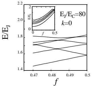
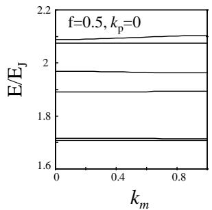
FIG. 4. The energy levels E vs. frustration and gate voltage for $\begin{array}{rlr}{E}_J/E_c& =& 80.\end{array}$ $\begin{array}{rlr}\alpha & =& 0.8,\end{array}$ and $\gamma =0.02$ . The gate voltage is related to the k values by $[k_P,k_m]=(\gamma C/2e)[V_A+V_B,V_A-V_B]$ , (a) $E/E_J$ vs $f_b$ near $f_b=1/2$ for $[k_p,k_m]=[0,0]$ , and (b) $E/E_J$ vs $k_m$ for $k_p=0.$

where the momenta can be written as $P_p=-i\hslash \partial /\partial {\phi }_p$ and $P_m=-i\hslash \partial /\partial {\phi }_m$ . The mass terms are $M_p=({\Phi }_o/2\pi {)}^{2}2C(1+$ $\gamma )$ and $M_m=({\Phi }_o/2\pi {)}^{2}2C(1+2\alpha +\gamma )$ . In this coordinate system the full wave function $\Psi ({\phi }_p,{\phi }_m)=\exp \{i(k_p^{\prime }{\phi }_p+$ $k_m^{\prime }{\phi }_m)\}\chi ({\phi }_p,{\phi }_m)$ with $[k_p^{\prime },k_m^{\prime }]=-(\gamma C/2e)[V_A+V_B,V_A-$ V_B] and $H_t\chi ({\phi }_p,{\phi }_m)=E\chi ({\phi }_p,{\phi }_m)$ . Also the two minima of the potential $U({\phi }_p,{\phi }_m)$ within a unit cell form a periodic two-dimensional centered cubic lattice with lattice constants ${\mathbf{a}}_1=2\pi {\mathbf{i}}_x$ and ${\mathbf{a}}_2=\pi {\mathbf{i}}_x+\pi {\mathbf{i}}_y.$

Fig. 4 shows the energy levels as a function of $f$ and as a function of the gate voltage which is given in terms of k. We have taken $E_J/E_c=80,\alpha =0.8$ , and $\gamma =0.02$ in this example. The energy levels are symmetric about $f=1/2$ . In Fig. 4a, we see that the two lowest energy levels near $f=1/2$ have opposite slopes, indicating that the circulating currents are of opposite sign. We also see that there is only a small range of $0.485<f<0.5$ where the qubit can be operated between these states of opposite circulating current. This range is consistent with the range $[\frac{1}{2}\pm f_c]$ from the classical stability as shown in Fig. 2. At $f=0$ .49 direct calculation of the average circulating current $,<\Psi |I_c$ sin ${\phi }_1|\Psi >$ gives that the circulating current for the lower level is $I_1/I_o=-0.70$ and for the upper level is $I_2/I_o=+0.70$ (A calculation of the circulating current from the thermodynamic relation $-{\Phi }_o^{-1}\partial E_n/\partial f$ gives the same result.) For a loop of diameter of $d=10\mu \mathrm{m}$ , the loop inductance is of the order ${\mu }_{o}d$ 10 pH [54]. For $I_o\approx 400\mathrm{nA}\left(E_J=200\mathrm{GHz}\right)$ , the flux due to the circulating current is $L{I}_1\approx 10^{-3}{\Phi }_o$ , which is detectable by an external SQUID. Nevertheless, the induced flux is small enough, that we are justified in neglecting its efect when calculating the energy levels.

The diference in energy between the lower and upper level at the operating point of $f=0.485$ is about $0.1EJ\approx 20\mathrm{GHz}$ Moreover, Fig. 4b shows that the energies of these levels is very insensitive to the gate voltages, or equivalently, to the random of-set charges. The numerical results show that the bands are flat to better than one part in a thousand, especially at $f=0.48$ . To understand the underlying physics, a tightbinding model is developed.

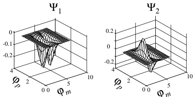
FIG. 5. The eigen wave functions for the lower $\left({\Psi }_1\right)$ and upper $\left({\Psi }_2\right)$ energy levels at $f=1/2$ as a function of the phases.

A. Tight-Binding Model

Consider the case near the degeneracy point $f=1/2$ . The minima in energy occurs when ${\phi }_p^{\ast }=0$ and ${\phi }_m=\pm {\phi }_m^{\ast }$ where cos ${\phi }_m^{\ast }=1/2\alpha$ . Near the minimum at $[{\phi }_m,{\phi }_p]=[{\phi }_m^{\ast },0]$ , the potential looks like a double potential well repeated at lattice points ${\mathbf{a}}_1=2\pi {\mathbf{i}}_x$ and ${\mathbf{a}}_2=\pi {\mathbf{i}}_x+\pi {\mathbf{i}}_y$ . Fig. 5 shows the two eigen functions in a unit cell. The wave function for the lower level $\left({\Psi }_1\right)$ is symmetric and the wave function for the upper level $\left({\Psi }_2\right)$ is antisymmetric. Both of the wave functions are localized near the two minima in $U$ in the unit cell.

To find an approximate tight-binding solution, let u \mathopen { } \mathclose \bgroup \left( \varphi _ { m } , \varphi _ { p } \aftergroup \egroup \right) be the wave function for the ground state on one side of the double potential wells, and v \mathopen { } \mathclose \bgroup \left( \varphi _ { m } , \varphi _ { p } \aftergroup \egroup \right) be the wave function on the other side. The tight-binding solution for $H_t$ in Eqn. 12 is $\Phi =c_{u}u+c_{v}v$ and satisfies

$$\left(\begin{array}{cc}{H}_{uu}& H_{uv}\\ H_{vu}& H_{vv}\end{array}\right)\left(\genfrac{}{}{0ex}{}{c_u}{c_v}\right)=E\left(\genfrac{}{}{0ex}{}{c_u}{c_v}\right)\text{\hspace{1em}(13)}$$

Because the double well is symmetric at $f=1/2,$ each wave function has the same energy ${ϵ}_0$ and so $H_{uu}=H_{vv}={ϵ}_0$ . Let $t_1$ be the tunneling matrix element between these two minima in the same unit cell and $t_2$ between nearest neighbor minima in the adjacent unit cells. Then $H_{uv}=H_{vu}^{\ast }=-t_1-t_2{e}^{i\mathbf{k}\cdot {\mathbf{a}}_2}-$ $t_2{e}^{i\mathbf{k}\cdot ({\mathbf{a}}_1-{\mathbf{a}}_2)}$ . The eigen energy levels are $E={ϵ}_0\mp |H_{uv}|$ . The efect of $t_1$ is to split the degeneracy of the two states so that at $k=0,$ the energy is ${ϵ}_0\mp \left(2t_2+t_1\right)$ for the symmetric and antisymmetric states respectively. The efect of $t_2$ is to give dispersion in $k,$ that is, in gate voltage and of-set charges, to the energy levels. Because we want to minimize the gatevoltage (and of-set charge) dependence, we seek to minimize the tunneling $t_2$ from one unit cell to another. Likewise, we want the two localized states in the two wells to interact, so that we want $t_1$ to be non-zero. This is why the potential landscape in Fig. 3 was chosen to have $\alpha \approx 0.8:$ The potential has a much lower barrier between states in the double well, but a large barrier between states from one double well to the next.

An estimate of $t_i$ can be obtained from calculating the action $S_i$ between the two minima and using $t_i$ ≈ $(\hslash {\omega }_i/2\pi )e^{-S_i/\hslash }$ where ${\omega }_i$ is the attempt frequency of escape in the potential well. The action from point ${\vec{\phi }}_a$ to ${\vec{\phi }}_b$ is

$$S={\int }_{\overrightarrow{{\phi }_a}}^{\overrightarrow{{\phi }_b}}{\left(2M_{nn}(E-U)\right)}^{1/2}|d{\phi }_n|\text{\hspace{1em}(14)}$$

Here n is a unit vector along the path of integration, $d{\phi }_n$ the diferential path length, and $M_{nn}={\mathbf{n}}^T\cdot \mathbf{M}\cdot \mathbf{n}$ is the component of the mass tensor along the path direction. In both cases we will approximate the energy diference $E-U$ as the diference in the potential energy $\Delta U$ from the minima along the path.

First, consider the calculation of $t_1$ , the tunneling matrix element within the unit cell. The path of integration is taken from $(-{\phi }_m^{\ast },0)$ to $({\phi }_m^{\ast },0)$ along the direction $\mathbf{n}={\mathbf{i}}_x$ , so that $M_{nn}=M_m$ for this path. The potential energy at the minima is $U_{min}=2-1/2\alpha .$ . The diference in the potential energy from the minima at $(-{\phi }_m^{\ast },0)$ along this path is can we written as $\Delta U_1=E_J\{2\alpha (\cos {\phi }_m-1/2\alpha {)}^2\}$ . The action along this path is then

$$S_1={\int }_{-{\phi }_m^{\ast }}^{{\phi }_m^{\ast }}(4M_m\alpha E_J{)}^{1/2}\left(\cos {\phi }_m-\frac{1}{2\alpha }\right)d{\phi }_m\text{\hspace{1em}(15)}$$

which yields

$$S_1=\hslash {\left[4\alpha (1+2\alpha +\gamma )E_J/E_c\right]}^{1/2}\left(\sin {\phi }_m^{\ast }-\frac{1}{2\alpha }{\phi }_m^{\ast }\right)\text{\hspace{1em}(16)}$$

Now consider $t_2,$ , the tunneling from unit cell to unit cell. For example, take the integration to be from $({\phi }_m^{\ast },0)$ to one of its nearest neighbor minima at $(\pi -{\phi }_m^{\ast },\pi )$ . We will take the path of integration to be a straight line joining these two points in the ${\phi }_m-{\phi }_p$ plane. This path is not the optimal trajectory, but the diference of this straight line path from the optimal trajectory is quadratic in the small deviations of these two paths. The straight line path is described by ${\phi }_m={\phi }_m^{\ast }+\lambda {\phi }_p$ where $\lambda =(\pi -2{\phi }_m^{\ast })/\pi ;$ it has a direction of $\mathbf{n}=\lambda {\mathbf{i}}_x+{\mathbf{i}}_y$ and a path length of ds $ds=\sqrt{1+{\lambda }^2}d{\phi }_p.$ The mass on this direction is $M_2=(M_p+{\lambda }^2{M}_m)/(1+{\lambda }^2)$ The diference of the potential energy along this path form the minima energy is $\Delta U_2/E_J=-2\cos {\phi }_p\cos \left({\phi }_m^{\ast }+\lambda {\phi }_p\right)+$ 2α cos² $({\phi }_m^{\ast }+\lambda {\phi }_p)+1/2\alpha$ . The action is then

$$S_2={\left[2M_2{E}_J(1+{\lambda }^2)\right]}^{1/2}{\int }_0^{\pi }{\left(\frac{\Delta U_2}{E_J}\right)}^{1/2}d{\phi }_p.\text{\hspace{1em}(17)}$$

The integrand is not analytically integrable, but it is zero at the end points of the integration and is well approximated by $\sqrt{\Delta U_2/E_J}\approx (1/\sqrt{2\alpha })\cos ({\phi }_p-\pi /2)$ . With this approximation, $S_2={\left(4M_2{E}_J(1+{\lambda }^2)/\alpha \right)}^{1/2}$ , which is

$$S_2=\hslash \sqrt{\frac{E_J}{E_c}\left(\frac{(1+\gamma )(1+{\lambda }^2)}{\alpha }+2{\lambda }^2\right)}.\text{\hspace{1em}(18)}$$

To compare the tunneling rates we would first need the attempt frequencies in the two directions. However, we can consider the attempt frequencies to be of the same order of magnitude and thus $t_2/\dot{t_1}\sim e^{-(S_2-S_1)/\hslash }$ . For $\alpha =0.8$ , we find that $S_1/(\hslash \sqrt{E_J/E_c})$ 0.6 and $S_2/(\hslash \sqrt{E_J/E_c})\approx 1.4$ For $E_J/E_c\sim 10\dot{0}$ , then $t_2/t_1\sim 10^{-4}\ll 1$ p. We are therefore able to ignore $t_2,$ the tunneling from the unit cell to unit cell. This means that there is little dispersion in the energy levels with k and consequently, with the voltage or of-set charges. In fact, using the action one can show that for α smaller than about 0.85, $t_1>t_2$ for $E_J/E_c\approx 80$ . Throughout the rest of the paper we will choose parameters so that the efects of $t_2$ can be ignored.

We now obtain an approximate solution for the energy levels and tunneling matrix elements by modeling each side of the double potential. Near the minimum at $[{\phi }_m,{\phi }_p]=[{\phi }_m^{\ast },0]$ 2 the potential looks like an anisotropic two-dimensional harmonic oscillator. The Hamiltonian in the vicinity of the minimum is approximately, (with $Q_i^I=0)$

$$\mathcal{H}\approx \frac{1}{2}\frac{P_p^2}{M_p}+\frac{1}{2}{M}_p{\omega }_p^2{\phi }_p^2+\frac{1}{2}\frac{P_m^2}{M_m}+\frac{1}{2}{M}_m{\omega }_m^2({\phi }_m-{\phi }_m^{\ast }{)}^2+U_0\text{\hspace{1em}(19)}$$

where

$$\frac{\hslash {\omega }_p}{E_J}=\sqrt{\frac{4}{\alpha (1+\gamma )(E_J/E_c)}}\text{\hspace{1em}(20)}$$

and

$$\frac{\hslash {\omega }_m}{E_J}=\sqrt{\frac{4(4{\alpha }^2-1)}{\alpha (1+2\alpha +\gamma )(E_J/E_c)}}\text{\hspace{1em}(21)}$$

and $U_o=2-1/2\alpha$ . The ground state ${\varphi }_o$ of the single harmonic well has energy ${ϵ}_0=\hslash ({\omega }_p+{\omega }_m)/2+U_o$ . Let’s now use this approximation to understand the energy levels, first at $f=1/2$ and then near this point.

$\mathrm{At}f=1/2$ we expect the four lowest energy levels of the two-dimensional harmonic oscillator to be with ${\omega }_m<{\omega }_p,$ $\begin{array}{r}{E}_1={ϵ}_0-t_1,E_2={ϵ}_0+t_1,E_3={ϵ}_0-t_1+\hslash {\omega }_m,E_4=\end{array}$ ${ϵ}_0+t_1+\hslash {\omega }_m$ . Table I compares the results and we also list the small anharmonic corrections to the simple harmonic energy levels. We have chosen to compare $(E_1+E_2)/2$ and $(E_3+E_4)/2$ so that the tunneling term is absent and a direct comparison with the simple harmonic oscillators can be made. The agreement between this tight-binding approximation and

	$\hslash {\omega }_m$	$\hslash {\omega }_p$	$E_0$	$(E_1+E_2)/2$	$(E_3+E_4)/2$
Harmonic	0.193	0.247	1.60	1.79	1.84
Anharmonic	0.183	0.238	1.59	1.77	1.83
Numerical	0.154	0.226	1.58	1.74	1.81

TABLE I. A comparison of the energy levels with the approximate harmonic oscillator levels (with harmonic and anharmonic terms) with the numerical calculations.Here, $f=1/2,\alpha =0.8,\gamma =0.02$ , and and $E_J/E_c=80$ . Also $U_o=1.38$ and $U_{\mathrm{bar}}=0.225$ for the harmonic and anharmonic estimations. All the energies are in units of $E_J$

the numerical calculations is good. We have also included the barrier height from one minimum to the other one in the same unit cell.

If we estimate the attempt frequency for $t_1$ as ${\omega }_m$ , then we find that for the parameters in Table I, that the action calculation gives $t_1=10^{-4}{E}_J$ . From the full wave functions, we estimate $t_1=(E_2-E_1)/2\approx 10^{-3}{E}_J$ . This discrepancy can be made smaller by noting that in the calculation of the action, we could more accurately integrate from the classical turning points in the potential rather than from the minima [55]. However, for our purposes, the action expression will be suficient for qualitative discussions, and we will use the full numerical calculations when estimating actual numbers.

So far we have estimated the energy levels and tunneling matrix elements when $f=1/2$ . As $f$ is decreased from $f=$ $1/2$ the potential U changes such that one well becomes higher than the other, and the barrier height also changes. For the qubit we are mainly interested in the lowest two energy states of the system, so we now estimate the terms in tight-binding expression of Eqn. 13. By defining the zero of energy as the average of the two lowest energy states at $f=1/2$ , we find that the Hamiltonian for these two states is

$$H=\left(\begin{array}{cc}F& -t\\ -t& -F\end{array}\right)\text{\hspace{1em}(22)}$$

Here F is the energy change of each of the wells measured with respect to the energy of the wells at the degeneracy point; that is, $F=(\partial U/\partial f)\delta f$ where $U$ is the potential energy energy. Note that since we will be operating the qubit just below the degeneracy point $f=1/2$ , then $F<0$ . Also, $t=t_1+\Delta t$ where $t_1$ is the intracell tunneling matrix element calculated at the degeneracy point and $\Delta t$ is the change. The eigen values are ${\lambda }_{1,2}=\mp \sqrt{F^2+t^2}$ where we have explicitly assumed that $F$ is negative and t is positive.

The eigen vectors are given as the columns in the rotation matrix

$$D(\theta )=\left(\begin{array}{cc}\cos \theta /2& -\sin \theta /2\\ \sin \theta /2& \cos \theta /2\end{array}\right)\text{\hspace{1em}(23)}$$

where $\theta :=:-$ arctan $t/F.$ . For example, at the degeneracy point, $F=0$ , so that $E=\mp t$ and the eigen vectors are $\overline{(1/\sqrt{2},1/\sqrt{2}{)}^T}$ and $(-1/\sqrt{2},1/\sqrt{2}{)}^T$ . These are just symmetric and antisymmetric combinations of the single well wave functions, as expected. For $f$ slightly below $1/2,$ we have $|F|\gg t,$ so $\theta \approx 0,$ and the energies are $E=\mp \sqrt{F^2+t^2}\approx \pm F$ The eigen vectors are approximately $(1,0{)}^T$ and $(0,1{)}^T$ , so that the eigen states are nearly localized in each well.

It is more convenient to discuss the Hamiltonian and eigen states in the rotated coordinate system such that $\begin{array}{rl}{H}_D& =\end{array}$ $D^T(\theta )HD(\theta )$ . In the rotated coordinate system, the Hamiltonian is diagonal with

$$H_D=-\sqrt{F^2+t^2}{\sigma }_z\text{\hspace{1em}(24)}$$

and the eigen energies are $E=\pm \sqrt{F^2+t^2}$ and the eigen states are then simply spin down $|0>=(1,0{)}^T$ and spin up $|1>=(0,1{)}^T$ vectors. In other words, no matter what the operating field is, we can always go to a diagonal representation; but the rotation matrix must be used to relate the simple spin up and down vectors to the linear combinations of the wave functions in the well.

V. MANIPULATION OF THE QUBIT

As noted above, the flexibility of the design of Josephson junction circuits afords a variety of methods for manipulating and controlling the state of qubits. In this section we show how the basic qubit circuit can be modified to allow precise control of its quantum states. To manipulate the states of the qubit, we need control over the properties of the qubit.

For example, control over $f,$ the magnetic field, allows one to change the operating point and $F,$ the value of the energy diference between the two states. Control over the potential barrier height allows changing of the tunneling through t. For example, if the operating point of $F_o$ and $t_o$ are changed by $\Delta F$ and $\Delta t.$ , then the Hamiltonian in the rotated coordinate system is

$$H_D=-\sqrt{F_o^2+t_o^2}{\sigma }_z+\Delta H_D\text{\hspace{1em}(25)}$$

where with ${\theta }_o=-\arctan t_o/F_o$

$$\Delta H_D=\Delta F(\cos \theta {\sigma }_z-\sin \theta {\sigma }_x)-\Delta t(\sin \theta {\sigma }_z+\cos \theta {\sigma }_x).\text{\hspace{1em}(26)}$$

The control over F can be done by changing $f.$ The control over t can be done by changing the barrier heights. $\mathrm{To}$ control the barrier heights by external parameters, we replace the third junction by a SQUID which acts like a variable strength junction. The modified circuit of the qubit is shown in Fig. 6.

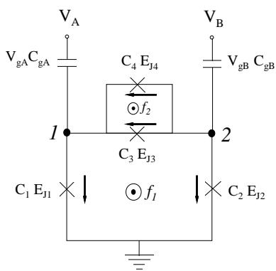
FIG. 6. The four-junction qubit. Two junctions form a SQUID loop and have Josephson Energies and capacitance $\beta$ times larger than the other junctions 1 and 2 which both have Josephson energies $E_J$ and capacitance $C.$ The nodes A and B represent the superconducting islands which are coupled by gate capacitors $C_g=\gamma C$ to gate voltages $V_A$ and $V_B$ . The arrows define the direction of the currents. The flux is out of the page.

We now analyze this circuit since it will be used in all subsequent discussion of the qubit. Flux quantization around each of the two loops, gives ${\phi }_1-{\phi }_2+{\phi }_3=-2\pi f_1$ and ${\phi }_4-{\phi }_3=-2\pi f_2$ . The Josephson energy due to each junction is $E_{Jn}(1-\cos {\phi }_n)$ . The total Josephson energy $U$ is then

$$\frac{U}{E_J}=2+2\beta -2\cos {\phi }_p\cos {\phi }_m-2\beta \cos (\pi f_a)\cos (2\pi f_b+2{\phi }_m),\text{\hspace{1em}(27)}$$

where ${\phi }_p=({\phi }_1+{\phi }_2)/2$ and ${\phi }_m=({\phi }_1-{\phi }_2)/2$ , and also $f_a=f_2$ and $f_b=f_1+f_2/2$ . Hence we see that $2\beta \cos (\pi f_a)$ plays the role of α in the three junction qubit, but now this term can be changed by changing $f_a=f_2$ , the flux in the top SQUID loop. Likewise, $f_b=f_1+f_2/2$ plays the role of $f$ in the three-junction qubit. The reduced Hamiltonian is then

$$\begin{array}{c}{H}_t=\frac{1}{2}\frac{P_p^2}{M_p}+\frac{1}{2}\frac{P_m^2}{M_m}+E_J\{2+2\beta \\ -2\cos {\phi }_p\cos {\phi }_m-2\beta \cos (\pi f_a)\cos (2\pi f_b+2{\phi }_m)\}\end{array}\text{\hspace{1em}(28)}$$

where $M_p=({\Phi }_o/2\pi {)}^{2}2C(1+\gamma )$ and $M_m=({\Phi }_o/2\pi {)}^{2}2C(1+$ $4\beta +\gamma )$ .

To manipulate the parameters in the Hamiltonian let the magnetic fields change very slightly away from the some degeneracy point of $f_1^{\ast }$ and $f_2^{\ast }$ to a new operating point $f_1^o=f_1^{\ast }+{ϵ}_1$ and $f_2^o=f_2^{\ast }+{ϵ}_2$ . Then F changes from zero to ${\mathbf{F}}_{\mathbf{o}}={\mathbf{r}}_1{\mathbf{ϵ}}_1+{\mathbf{r}}_2{\mathbf{ϵ}}_2$ and t changes to $t_o=t_1+s_1{ϵ}_1+s_2{ϵ}_2$ , where $r_i$ and $s_i$ are constants and $t_1$ is the tunneling matrix element at the degeneracy point as found in the previous section. We take the operating point to be efectively in the regime where $f<1/2$ in Fig. 4, so that ${ϵ}_{1,2}<0$ . Hence, $F_o<0$ . Also, $t_o$ is assumed to remain positive. In the new rotated frame with ${\theta }_o=-\arctan t_o/F_o$ , the Hamiltonian given by Eqn. 24 is $H_D=-\sqrt{F_o^2+t_o^2}{\sigma }_z$

Away from this new operating point, let $f_1=f_1^o+{\delta }_1$ and $f_2=f_2^o+{\delta }_2$ . In the operation of the qubit, $\left|{\delta }_i\right|\ll \left|{ϵ}_i\right|$ and ${\delta }_i$ usually will usually have a sinusoidal time dependence. Then $F=F_o+r_1{\delta }_1+r_2{\delta }_2$ and $t=t_o+s_1{\delta }_1+s_2{\delta }_2$ , so that $\Delta F=$ $r_1{\delta }_1+r_2{\delta }_2$ and $\Delta t=s_1{\delta }_1+s_2{\delta }_2$ . Then Hamiltonian in the rotated system with θ = arctan $t_o/F_o$ is

$$H_D=-\sqrt{F_o^2+t_o^2}{\sigma }_z+\Delta H_D\text{\hspace{1em}(29)}$$

where

$$\begin{array}{rl}\Delta H_D=& (r_1{\delta }_1+r_2{\delta }_2)(\cos {\theta }_o{\sigma }_z-\sin {\theta }_o{\sigma }_x)\\ & -(s_1{\delta }_1+s_2{\delta }_2)(\sin {\theta }_o{\sigma }_z+\cos {\theta }_o{\sigma }_x).\end{array}\text{\hspace{1em}(30)}$$

Hence we see that changes in the magnetic field from the operating point of $f_1^o$ and $f_2^o$ cause both ${\sigma }_z$ and ${\sigma }_x$ types of interactions.

To find the magnitude of these changes, we calculate the coeficients of change $(r_1,r_2,s_1$ and ${}^{s_2)}$ most simply at the degeneracy point where ${ϵ}_i=0;$ ; that is, at the degeneracy point $f_i^o=f_i^{\ast }$ . We choose the degeneracy point for the fourjunction qubit at $f_1^{\ast }=1/3$ and $f_2^{\ast }=1/3$ . This results in classically doubly degenerate levels. In fact, any choice which satisfies $2f_1^{\ast }+f_2^{\ast }=1$ when the classical energy U has two minima, will also result in doubly degenerate levels. For example $f_1^{\ast }=1/2$ and $f_2^{\ast }=0$ is also a possible and convenient choice. However, we prefer $f_1^{\ast }=f_2^{\ast }=1/3$ for the following reason. The change in potential energy with $f_a$ gives

$$\begin{array}{r}\frac{\partial U}{\partial f_a}=-2\pi \beta \sin \pi f_a\cos 2{\phi }_m^o\\ \frac{{\partial }^{2}U}{\partial f_a^2}=-2{\pi }^2\beta \cos \pi f_a\cos 2{\phi }_m^o\end{array}\text{\hspace{1em}(31)}$$

The first order terms vanishes if $f_2^o=0,$ , resulting in the potential barrier always decreasing with changes in $f_2.$ . On the other hand, if $f_2^o=1/3$ , then the barrier height can be made to increase and decrease with changes in $f_2$ , thus allowing more control of the qubit.

Now the coeficients of change $(r_1,r_2,s_1$ and $s_2)$ can be estimated both from the numerical calculations and from the tight-binding model as shown in Appendix B. We find that at the degeneracy point of $f_1=f_2=1/3$ 2

$$\frac{r_1}{E_J}=2\pi \sqrt{1-1/(4{\beta }^2)}.\text{\hspace{1em}(32)}$$

For our example with $\beta =0.8,$ we have $r_1/E_J=4.90$ . Estimates obtained from the numerical calculations done by changing $f_1$ and $f_2$ , give $r_1/E_J=4.8$ and $r_2/E_J=2.4$ in good agreement with Eqn. 56 in Appendix B.

Likewise, from Appendix B we have that $s_1=0$ and $s_2=$ ηt $\sqrt{E_J/E_c}$ where η is of the order of unity. For the operating ppoint we find $\eta \sim 3.5$ . Therefore, changes in H due to changes in t₁ go like ${\sigma }_x.$ . These tight-binding estimates for $\beta =0.8$ give $s_1=0$ and $s_2/E_J=0.03$ . Full numerical calculations for our example with $s_1=0$ and $s_2/E_J=0.20$ . The agreement with the tight-binding results are good, although the tight-binding underestimates $s_2$ with for these parameters.

In summary, from the degeneracy point of $f_1^{\ast }=f_2^{\ast }=1/3$ 2 let the operating point be $f_1^o=f_1^{\ast }+{ϵ}_1$ and $f_2^o=f_2^{\ast }+{ϵ}_2$ so that $F_o=r_1({ϵ}_1{ϵ}_2/2)$ and $t_o=t_1+s_2{ϵ}_2$ . Now consider the changes in field about the operating point such that $f_1=$ $f_1^{\ast }+{\delta }_1$ and $f_2=f_2^{\ast }+{\delta }_2$ . In the rotated frame where ${\theta }_o=$ arctan $t_o/F_o.$ , the Hamiltonian is

$$H_D=-\sqrt{F_o^2+t_o^2}{\sigma }_z+\Delta H_D\text{\hspace{1em}(33)}$$

where

$$\begin{array}{rl}\Delta H_D=& r_1({\delta }_1+\frac{{\delta }_2}{2})(\cos {\theta }_o{\sigma }_z-\sin {\theta }_o{\sigma }_x)\\ & -s_2{\delta }_2(\sin {\theta }_o{\sigma }_z+\cos {\theta }_o{\sigma }_x).\end{array}\text{\hspace{1em}(34)}$$

and $r_1/E_J=2\pi \sqrt{1-1/(4{\beta }^2)}\mathrm{and}{s}_2=\eta t_o\sqrt{E_J/E_c}.$

pA typical design for a qubit will have $E_J/\dot{E_c}=80,\beta =0.8,$ 2 $\gamma =0.02$ . We find from numerical calculations that $t_o$ ≈ $0.005E_J$ and $\eta \approx 3.5$ , which agree well with our tight-binding estimates. We operate at $f_1=f_2=0.33$ so that ${ϵ}_1={ϵ}_2=$ $-1/300$ . (This is equivalent to operating the three-junction qubit at $f=f_1+f_2/2=0.495$ in $Fig.4.)$ Writing the energies as $E_i=h{\nu }_i$ , we have taken typical values of $E_J=200$ GHz and $E_c=2.5\mathrm{GHz},$ and we find that $t_o=1\mathrm{G}$ Hz and $F_o=$ 5 GHz (which gives a splitting between the two states of about 10 GHz). The Hamiltonian is found to be

$$\frac{H_D}{E_J}=-0.025{\sigma }_z+(4.0{\delta }_1+2.1{\delta }_2){\sigma }_z-(0.46{\delta }_1+0.41{\delta }_2){\sigma }_x\text{\hspace{1em}(35)}$$

The numerical values used are from numerical calculations. These values agree well with the estimates used in Eqns. 33 and 34 for the level splitting and the terms proportional to $r_1;$ the terms proportional to $s_2$ match to about 50%, due to the more sensitive nature of estimating the tunneling terms.

The terms containing ${\sigma }_x$ can be used to produce Rabi oscillations between the two states by modulating ${\delta }_1$ and ${\delta }_2$ with microwave pulses of the frequency of the level splitting of $2F_o=10\mathrm{GHz}$ . One could arrange the values of ${\delta }_1$ and ${\delta }_2$ to make the time-varying ${\sigma }_z-\mathrm{term}$ vanish. Then the operation of the qubit would be isomorphic to the NMR qubit. However, our simulations show that such an arrangement couples higher energy levels and invalidates the simple two-state approximation. This is due to the large matrix element between the ground state and the second excited state given by the change in potential due to varying ${\delta }_2$ . (It is interesting to note that similar coupling to higher levels occurs in qubits based on the RF SQUID and on simple charge states.) We propose to manipulate the qubit by varying δ₁ which causes a Rabi oscillation through the ${\sigma }_x$ term as well as a strong modulation of the Larmor precession through the time varying ${\sigma }_z$ term. Because the Rabi frequency is much smaller than the Larmor frequency, the precession causes no problem for manipulating the qubit. For ${\delta }_1=0.001$ and ${\delta }_2=0$ , the Rabi frequency is about 90 MHz. We note that this mode of operation is also possible with the three-junction qubit. Of course, it will not be possible to completely eliminate the deleterious efects of the ${\delta }_2$ coupling, but the efect of this coupling can be greatly reduced if ${\delta }_2$ is restricted below 0.0001.

(a)

(b)
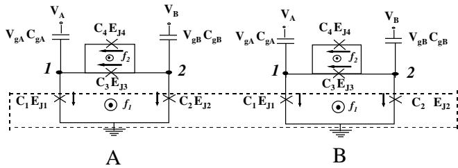
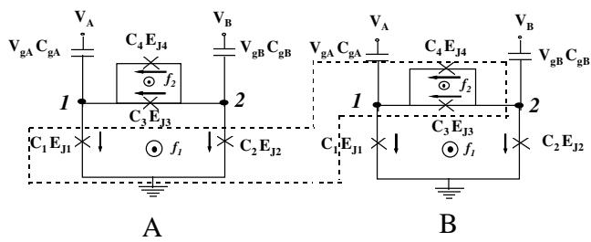
FIG. 7. Coupling of qubits A and B through the mutual inductance between (a) the lower regions of both, and (b) the lower region of A and the upper region of B.

The varying magnetic fields ${\delta }_1$ and ${\delta }_2$ can be applied locally to the qubit by using a control line to inductively couple to the qubit. Moreover, if the the control line is driven by an Josephson oscillator, then the coupling circuit could be fabricated on the same chip.

VI. INTERACTION BETWEEN QUBITS

A variety of methods are available for coupling qubits together. As noted in [13,14], essentially any interaction between qubits, combined with the ability to manipulate qubits individually, sufices to construct a universal quantum logic gate. Here we present two methods for coupling qubits inductively as shown in Fig. 7. The inductive coupling could either be permanent, or could be turned on and of at will by inserting Josephson junctions in the coupling loops.

Fig. 7a shows one way of coupling two identical qubits. The lower portions of each qubit (the loops that contain the circulating currents) are inductively coupled. To a first approximation we model the coupling as changing the flux in each of the two lower rings only through the mutual inductive coupling. (We ignore the the self-inductance which can easily be included.) The efective frustration in the lower loop of $A,{\tilde{f}}_1^A$ , is changed over the applied frustration $f_1^A$ to ${\tilde{f}}_1^A=f_1^A+M{I}_1^B/{\Phi }_o$ Here the current in the lower loop of $B$ is $I_1^B$ . Similarly, ${\tilde{f}}_1^B=f_1^B+M{I}_1^A/{\Phi }_o$ . The coupled Hamiltonian is

$$H_{AB}=H^A(\widetilde{f_1^A})+H^B(\widetilde{f_1^B})+M{I}_1^A{I}_1^B\text{\hspace{1em}(36)}$$

which is the sum of the Hamiltonians for each system plus a term due to the mutual inductive coupling.

The inductively coupled contribution to the frustration is estimated to be of the order of $10^{-3}{\Phi }_c$ which is much smaller than the applied frustration. Since each persistent current will inductively couple into the other qubit, this will produce changes in the Hamiltonian of the ${\sigma }_z$ and ${\sigma }_x$ type and these changes will be proportional to the sign of the circulating currents in the qubit. Hence, we expect the coupling to be described by an interaction Hamiltonian of the form,

$$H_{AB}^{\mathrm{int}}={\kappa }_1{\sigma }_z^A{\sigma }_z^B+{\kappa }_2{\sigma }_z^A{\sigma }_x^B++{\kappa }_3{\sigma }_x^A{\sigma }_z^B\text{\hspace{1em}(37)}$$

Hence we see that this interaction has both $\mathrm{a}{\sigma }_z^A{\sigma }_z^B$ and $\mathrm{a}$ ${\sigma }_z^A{\sigma }_x^B$ types of coupling. We have estimated magnitude of ${\kappa }_i\approx 0.01E_J$

As Eqn. 35 shows, the inductive coupling between the qubits can be made to be a substantial fraction of the qubit Larmor frequency. This is an attractive feature, as the coupling between two qubits sets the speed limit for how rapidly two qubit quantum logic operations can be performed in principle. In practice, it may be desirable to sacrifice speed of operation for enhanced accuracy: in this case, the inductive coupling could be designed to be smaller by decreasing the overlap of the inductive loops with the circuits.

Coupling between qubits is similar to the coupling we envision between the qubit and the measurement circuits containing SQUID-like detectors. In its usual configuration, the SQUID is biased in the voltage state which produces a voltage related to the flux through its detector loop. However, such a strong, continuous measurement on a qubit would destroy the superposition of states in the qubit and project out only one of the states. This problem can be circumvented by designing a SQUID such that it is current biased in the superconducting state and hence is not measuring the flux in its detector loop. When one needs to measure the qubit, the SQUID can be switched to its voltage state, for example, by applying a pulse of bias. The coupling from mutual inductance between the SQUID and the qubit will also have to be controlled. Other measurement schemes using SQUIDs which are weakly coupled to the macroscopically coherent system have been proposed [56].

VII. COMPUTING WITH THE PC QUBIT

All the ingredients for quantum computation are now available. We have qubits that can be addressed, manipulated, coupled to each other, and read out. As will be indicated below, the particular qubits that we have chosen are well insulated from their environment as well. The flexibility of design for collections of qubits now allows a wide variety of overall designs for quantum computers constructed from such qubits.

Before discussing various superconducting quantum computer architectures, let us review some basic ideas about quantum logic and see how to implement quantum logic using our superconducting qubits. A quantum logic gate is a unitary operation on one or more qubits. Quantum computations are typically accomplished by building up quantum logic circuits out of many quantum logic gates. Just as in the case of classical computers, certain sets of quantum logic gates are universal in the sense that any quantum computation can be performed by wiring together members of the set. In fact, almost any interaction between two or more qubits is universal [13,14]; but a convenient universal set of quantum logic gates widely used in the design of quantum algorithms consists of single qubit rotations and the quantum controlled-NOT gate, or CNOT [57].

A. One-Qubit Rotation

An arbitrary one qubit rotations can be written as $e^{-i\sigma t}=$ cos t i sin t σ for some Pauli matrix $\sigma =a{\sigma }_x+b{\sigma }_y+c{\sigma }_z$ where $a^2+b^2+c^2=1$ . There are many ways of accomplishing a one qubit rotation: the ability to rotate the qubit by a precise amount around any two orthogonal axes sufices. Pursuing the analog with NMR, we choose a method that involves applying an oscillatory field applied at the qubit’s resonant frequency to rotate the qubit.

The Hamiltonian for a single qubit (A) can be gotten from Eqn. 35. Here we assume $E_J=200\mathrm{GHz},{\delta }_1=0.001$ cos ωt and ${\delta }_2=0$ , and the level splitting is $\omega =10\mathrm{GHz}$ . Then, the Hamiltonian is

$$H_D(\mathrm{GHz})=5{\sigma }_z+0.80(\cos \omega t){\sigma }_z-0.09(\cos \omega t){\sigma }_x\text{\hspace{1em}(38)}$$

The Rabi frequency is 90 $MHz$ so that a π pulse would be about 20 nsec.

B. Two-Qubit Controlled NOT

A controlled NOT is a two qubit quantum logic gate that flips the value of the second qubit if the value of the first qubit is 1. That is, it takes: $|00⟩|00⟩,|01⟩|01⟩,|10⟩|11⟩$ and $|11⟩|10⟩$ . A controlled NOT can be combined with single qubit rotations to give arbitrary quantum logic operations. A controlled NOT can be straightforwardly implemented in the superconducting qubit system by exploiting the analogy with NMR. Suppose that two qubits A and B have been constructed with an inductive coupling between their lower loops as in the first part of the previous section. Then the level splitting of qubit B depends on the state of qubit A, with values $\Delta E_{A,0}$ for A in the $|0>$ state and $\Delta E_{A,1}$ for A in the 1 > state. When a resonant pulse corresponding of $\Delta E_{A,1}/\hslash$ is applied to qubit $B,$ it will only change if qubit A is in its $|1>$ state. Since the coupling between the qubits is considerably larger than the Rabi frequency, the amount of time that it takes to perform the controlled NOT operation is equal to the amount of time it takes to perform a π rotation of a single qubit.

So the basic quantum logic operations can be performed on our superconducting qubits in a straightforward fashion. Accordingly, it is possible in principle to wire groups of qubits together to construct a quantum computer. A variety of architectures for quantum computers exist, usually consisting of regular arrays of quantum systems that can be made to interact either with their neighbors or with a quantum “bus” such as a cavity photon field or a phonon field in an ion trap that communicates equally with all the systems in the array. Because of the flexibility inherent in laying out the integrated Josephson junction circuit, a wide variety of architectures are possible. A particularly simple architecture for a quantum computer can be based on the proposal of Lloyd [1,5] for arrays of quantum systems such as spins or quantum dots.

C. Linear Chain of Qubits

Consider a linear array of qubits $ABABABAB\dots$ . Let the bottom of each qubit be inductively coupled to the top of the neighbor to the left. Also let each type of qubit, A and $B,$ have a slightly diferent Josephson energy. Each qubit also has the area of the top loop which is half that of the bottom loop. In the absence of the driving electromagnetic fluxes (the ${\delta }_i^j)$ , the Hamiltonian for the system can be generalized to be written as

$$H=-\hslash \sum _k\left({\omega }_k{\sigma }_k^z+2J_{k,k+1}{\sigma }_k^z{\sigma }_{k+1}^z\right)\text{\hspace{1em}(39)}$$

where $\hslash {\omega }_k=\sqrt{F_k^2+t_k^2}$ and $J_{k,k+1}={\kappa }_{k,k+1}(r_{1,k}+r_{1,k+1})/2$ pThis problem then maps on the linear chain of nuclear spins which was shown by Lloyd [5] to be a universal quantum computer. The coupling needed to perform $\pi /2$ pulses is provided by the terms containing the ${\delta }_i^j{}^{,}\mathrm{s}.$ The nice feature of this linear chain is that separate control lines for AC fields are not needed. The whole linear array can sit in a microwave cavity and be pulsed at the desired frequency. (The dc bias fields to ensure $f_1=f_2=1/3$ will require at least two dc control lines). The frequencies needed are around 10—25 GHz with intervals of 1 GHz (and with resolution of about 0.1 GHz). We could make these numbers larger or smaller if needed.

Details of computing with this are given in various references, see for examples Ref. [5] and Chapter 20 of Ref. [58].

D. Superconducting Quantum Integrated Circuits

There is no reason why the inductive loops cannot couple qubits that are far apart. In addition, a single qubit can be coupled to several other qubits as shown in Fig. 8. This arrangement requires separate AC control lines for each of the qubits, which then demands localized on-chip oscillators. One can build up essentially arbitrary integrated circuits of superconducting qubits by this method. This flexibility in the construction of quantum computer architectures is one of the benefits of using superconducting Josephson junction circuits to perform quantum computation. The quantum integrated circuit could be set up to provide a number of useful features. For example [59], one might be able to design the circuit and interactions in such a way that it automatically implements an intrinsically fault-tolerant quantum computer architecture such as those proposed by Kitaev [60] and Preskill [61]. In addition, since the circuits are parallelizable in that diferent quantum logic operations can be performed in diferent places simultaneously, the circuit could be designed to provide the maximum possible parallelization of a particular problem such as factoring [62], database search [63], or computing a discrete quantum Fourier transform [62,64].

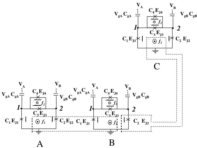
FIG. 8. A method for coupling a single qubit to other qubits.

VIII. DECOHERENCE

We have shown how superconducting circuits can be used to construct qubits and quantum logic circuits. These superconducting qubits have been idealized in the sense that we have ignored the efects of manufacturing variability, noise and decoherence. Manufacturing variability can be compensated for as discussed above: before performing any quantum computations, the properties of individual qubits can be measured, recorded in a look-up table in a conventional computer, and used either to supply compensating calibration fields or to alter the frequencies with which control pulses are supplied to the qubits.

From the point of view of the ultimate performance of a superconducting computer, a more pressing issue is that of environmentally induced noise and decoherence. In real systems the performance of a qubit will be limited by dissipative mechanisms which cause the quantum state to decohere in time ${\tau }_d.$ . The ‘quality factor’ for a qubit is the decoherence time divided by the amount of time it takes to perform fundamental quantum logic operations [3]. The quality factor gives the number of quantum logic operations that can be performed before the computation decoheres, and should be $10^4$ or greater for the quantum computer to be able to perform arbitrarily long quantum computations by the use of error-correction techniques [65–69].

Decoherence can be due to “internal” dissipation (quasiparticle resistance), or coupling to an environmental degree of freedom. It is also possible to couple to an environmental degree of freedom, without a dissipative mechanism, that will still lead to decoherence [70]

We will now discuss some of the major sources of decoherence.

Normal state quasi-particles can cause dissipation and energy relaxation at finite temperatures in Josephson junctions. However, mesoscopic aluminum junctions have been shown to have the BCS temperature dependence for the density of quasi-particles. At low temperatures this density is exponentially small [71], so quasi-particle tunneling will be strongly suppressed at low temperatures and at low voltages, as was seen in a system with multiple superconducting islands in Ref. [72]. We estimate a lower bound of $10^4$ for the quality factor, given a sub-gap resistance of $10^{10}\Omega [71]$

The qubit can also decohere by emitting photons. We estimate this by classically estimating the rate photons are emitted by magnetic dipole radiation from oscillating current in the loop defining the qubit. For a loop with radius R with an alternating current of frequency ν and rms amplitude of $I_m,$ , the power transmitted to free space is $P_m=K_m{R}^4{I}_m^2{\nu }^4$ where $K_m=8{\mu }_o{\pi }^5/3c^3$ . A typical rate for photon emission is $1/t_m=P_m/h{\nu }_{;}$ , which gives an estimate of the decoherence time of $t_m=h/K_m{R}^4{I}_m^2{\nu }^3$ . An estimate for the frequency is the Larmor frequency, (other characteristic frequencies such as the Rabi frequency are even smaller). For our qubit $R\approx 1\mu \mathrm{m},\nu \approx 10\mathrm{GHz}$ and $I_m=1\mathrm{nA}$ , we find that $t_m\sim 10^7\mathrm{s}$ , so that this is not a serious source of decoherence. However, it should be noted that proposals for using RF SQUIDs for qubits, involve currents of the order of $1\mu \mathrm{A}$ and and loops of the order of $10\mu \mathrm{m}$ . These RF SQUIDs have $t_m\approx 10^{-3}\sec$ , which is substantially lower than for our qubits which can be made much smaller have much less current.

Inhomogeneity in the magnetic flux distribution can also be a source of decoherence. This is similar to $T_2$ in NMR systems. We estimate this for our system by calculating the amount of flux a $1\mu \mathrm{m}\times 1\mu \mathrm{m}$ wire carrying 100 nA of current induces in a loop of the same size which has its center 3 µm away. We find that the induced frustration is about $\delta f=10^{-7}$ If this is taken as an estimate of the typical variance of the frustration that diference qubits experience, then there will be a spread of operating frequencies among the loops. An estimate of $t_d$ is the time for the extremes of this frequency difer by $\pi .$ . This results in $t_d\approx \pi /(2r_1\delta f)$ , where we have taken the larger value from Eqn. 35. With $r_1/\hslash \approx 600\mathrm{GHz}$ we find $t_d\approx 1.5$ msec. The dipole-dipole interaction between qubits gives a time of the same order.

We have also estimated the magnetic coupling between the dipole moment of the current loops and the magnetic moments of the aluminum nuclei in the wire. At low temperatures where the quasi-particles are frozen out, the decoherence time for a single qubit is of the order of $T_1$ which is exponentially large in the low-temperature superconducting state. For an ensemble of qubits, the decoherence time time may be of the order of milliseconds due to the diferent configurations of nuclear spins in the diferent qubits. However, this efect may be reduced by aligning the spins or by applying compensating pulse sequences.

Coupling to ohmic dissipation in the environment has been modeled for superconducting qubits operating in the charging regime [19]. They found that source of decoherence could be made suficiently small such that the quality factor is large enough. Similar calculations for qubits in the superconducting regime of circulating currents have not yet been done. Experiments to measure this decoherence time in our circuits are underway. In practice electromagnetic coupling to the normal state ground plane can limit coherence [35]; however, a superconducting ground plane can greatly reduce this coupling.

Other possible sources of decoherence are the efects of the measuring circuit, the arrangement and stability of the control lines for the magnetic fields, the ac dielectric losses in the substrate at microwave frequencies. These and other source of decoherence will have to be estimated in a real circuit environment and measured.

Taking 0.1 msec as a lower bound on the decoherence time and 10 nsec as a switching time, we find that the quality factor is of the order of $10^4$ . Furthermore, if the proper set of topological excitations is used to store information, the decoherence time for quantum computation can be made substantially longer than the minimum decoherence time for an individual junction circuit [60].

IX. SUMMARY

In this paper we have discussed a superconducting qubit which has circulating currents of opposite sign as its two logic states. The circuit consist of three nano-scale Josephson junctions connected in a superconducting loop and controlled by magnetic fields. One of the three junctions is a variable junction made as a SQUID loop. This qubit has quantum states which are analogous to a particle with an anisotropic mass moving in an two-dimensional periodic potential. Numerical calculations of the quantum states of the qubit have been made as well as physical estimates from a tight-binding approximation. The advantages of this qubit is that it can be made insensitive to background charges in the substrate, the flux in the two states can be detected, and the states can be manipulated with magnetic fields. Coupled systems of qubits are also discussed as well as sources of decoherence.

ACKNOWLEDGMENT

This work is supported by ARO grant DAAG55-98-1-0369. TPO acknowledges support from the Technical University of Delft and the Center for Superconductivity at the University of Maryland where part of this work was done. JJM is supported by the Fulbright Fellowship and from DGES (PB95- 0797). The work in Delft is financially supported by the Dutch Foundation for Fundamental Research on Matter (FOM). We thank Kostya Likharev, Kees Harmans, Peter Hadley, Chris Lobb, Fred Wellstood, and Ton Wallast for stimulating and useful discussions.

In this appendix we find the eigen values of the stability matrix for the three junction potential and the range of frustration around $f=1/2$ where there are two stable classical solutions with opposite circulating currents.

The potential energy of the Josephson energy of the three junction qubit is given by Eqn. 1

$$\tilde{U}=\frac{U}{E_J}=2+\alpha -\cos {\phi }_1-\cos {\phi }_2-\alpha \cos (2\pi f+{\phi }_1-{\phi }_2)\text{\hspace{1em}(40)}$$

We are interested in minimum energy phase configurations; that is, stable solutions of the following system of equations:

$$\begin{array}{rl}& \frac{\partial \tilde{U}}{\partial {\phi }_1}=\sin {\phi }_1+\alpha \sin (2\pi f+{\phi }_1-{\phi }_2)=0\\ & \frac{\partial \tilde{U}}{\partial {\phi }_2}=\sin {\phi }_2-\alpha \sin (2\pi f+{\phi }_1-{\phi }_2)=0\end{array}\text{\hspace{1em}(41)}$$

The solutions $({\phi }_1^{\ast },{\phi }_2^{\ast })$ complies with: sin ${\phi }_1^{\ast }=-\sin {\phi }_2^{\ast }=$ sin ${\phi }^{\ast }$ . Then

$$\sin {\phi }^{\ast }=-\alpha \sin (2\pi f+2{\phi }^{\ast })\text{\hspace{1em}(42)}$$

In order to check the character of the solution we compute the eigen values of the stability matrix, $\frac{{\partial }^2\tilde{U}}{\partial {\phi }_i\partial {\phi }_j}$ , where

$$\begin{array}{c}\frac{{\partial }^2\tilde{U}}{\partial {\phi }_1^2}=\cos {\phi }_1+\alpha \cos (2\pi f+{\phi }_1-{\phi }_2)\\ \frac{{\partial }^2\tilde{U}}{\partial {\phi }_2^2}=\cos {\phi }_2+\alpha \cos (2\pi f+{\phi }_1-{\phi }_2)\\ \frac{{\partial }^2\tilde{U}}{\partial {\phi }_1\partial {\phi }_2}=-\alpha \cos (2\pi f+{\phi }_1-{\phi }_2)\end{array}\text{\hspace{1em}(43)}$$

For the states with cos ${\phi }_1^{\ast }=\cos {\phi }_2^{\ast }=\cos {\phi }^{\ast }$ (these are the ones we are interested here), the eigen values are

$$\begin{array}{l}{\lambda }_1=\cos {\phi }^{\ast }\\ {\lambda }_2=\cos {\phi }^{\ast }+2\alpha \cos (2\pi f+2{\phi }^{\ast })\end{array}\text{\hspace{1em}(44)}$$

When $f\ne 0,1/2$ we have used relaxation methods for computing ${\phi }^{\ast }$ . Both eigen values are greater than zero which assures the minimum energy condition. Fig. 2 shows the energy of the minimum energy configurations for $\alpha =\mathrm{0.8.}$ . We find that there exists a region of values of the field for which two diferent minimum energy phase configuration coexist.

Next we calculate the critical values of the external field for this coexistence. We can restrict our analysis to the region around $f=0.5;$ that is, $[0.5-f_c,0.5+f_c]$ (where $f_c\ge 0)$ These extrema values of the field correspond to solutions for which one of the eigen values is positive and the other equals zero. The inset of Fig. 2 shows $f_c(\alpha )$

We first calculate $f_c$ when $\alpha \ge 1.0$ . The first eigen value which equals zero is ${\lambda }_1$ . Then at $f=0.5\pm f_c,{\lambda }_1=0$ which implies ${\phi }^{\ast }=\mp \pi /2$ mod 2π (here and below we associate the sign in $f_c$ with the sign of the phase in order to have $f_c\ge 0)$ Then, going to Eqn. 42 we get

$$\begin{array}{r}\sin (\mp \pi /2)=-\alpha \sin (\pi \pm 2\pi f_c\mp \pi )\\ \pm 1=\pm \alpha \sin (2\pi f_c)\end{array}\text{\hspace{1em}(45)}$$

and

$$f_c=\frac{1}{2\pi }\arcsin \frac{1}{\alpha }.\text{\hspace{1em}(46)}$$

We now calculate $f_c$ when $0.5\le \alpha \le 1.0$ . Now the first eigen value to equal zero is ${\lambda }_2$ , and we have to solve:

$$\begin{array}{l}\sin {\phi }^{\ast }=-\alpha \sin (2\pi f+2{\phi }^{\ast })=\alpha \sin (\pm 2\pi f_c+2{\phi }^{\ast })\\ \cos {\phi }^{\ast }=-2\alpha \cos (2\pi f+2{\phi }^{\ast })=2\alpha \cos (\pm 2\pi f_c+2{\phi }^{\ast })\end{array}\text{\hspace{1em}(47)}$$

We will use $\Delta =\pm 2\pi f+2{\phi }^{\ast }$ , so that

$$\begin{array}{rl}& 1={\sin }^2{\phi }^{\ast }+{\cos }^2{\phi }^{\ast }\\ & ={\alpha }^2{\sin }^2\Delta +4{\alpha }^2{\cos }^2\Delta \\ & ={\alpha }^2+3{\alpha }^2{\cos }^2\Delta \end{array}\text{\hspace{1em}(48)}$$

Then

$$\cos \Delta =\sqrt{\frac{1-{\alpha }^2}{3{\alpha }^2}};\Delta =\mp \arccos (\sqrt{\frac{1-{\alpha }^2}{3{\alpha }^2}})$$ $$\cos {\phi }^{\ast }=2\sqrt{\frac{1-{\alpha }^2}{3}};{\phi }^{\ast }=\mp \arccos (2\sqrt{\frac{1-{\alpha }^2}{3}})\text{\hspace{1em}(49)}$$

Here we have followed the solution corresponding to cos $\left({\phi }^{\ast }\right)\ge$ 0. Finally we have the solution for $f_c(\Delta =\pm 2\pi f_c+2{\phi }^{\ast })$

$$f_c=\frac{1}{2\pi }\left[2\arccos (2\sqrt{\frac{1-{\alpha }^2}{3}})-\arccos (\sqrt{\frac{1-{\alpha }^2}{3{\alpha }^2}})\right]\text{\hspace{1em}(50)}$$

APPENDIX B: TIGHT-BINDING ESTIMATE OFCOEFFICIENTS OF CHANGE

Recall that $f_a=f_2$ and $f_b=f_1+f_2/2$ . Assume that we change $f_a$ and $f_b$ independently. The minima in U occur at ${\phi }_p^{\ast }=0$ and ${\phi }_m^{\ast }=\pm {\phi }_m^o$ Therefore, the energy due to the potential energy is for each of the minimum

$$\frac{U}{E_J}=2+2\beta -2\cos {\phi }_m^{\ast }-2\beta \cos (\pi f_a)\cos (2\pi f_b+2{\phi }_m^{\ast }).\text{\hspace{1em}(51)}$$

The change in the magnetic flux $f_a$ by $\delta f_a$ causes a change in $U$ of

$$\frac{\partial U}{\partial f_a}\delta f_a=-2\pi \beta \sin \pi f_a\cos 2{\phi }_m^o\delta f_a\text{\hspace{1em}(52)}$$

which is the same for the minimum $\mathrm{at}\pm {\phi }_m^o$ . Whereas, the flux $f_b$ causes a change

$$\frac{\partial U}{\partial f_b}\delta f_b=\mp 4\pi \beta \cos \pi f_a\sin 2{\phi }_m^o\delta f_b\text{\hspace{1em}(53)}$$

which has opposite signs for the two minimum. Therefore,

$$\frac{\Delta U}{E_J}=-2\pi \beta \sin \pi f_a\cos 2{\phi }_m^o\delta f_{a}1-4\pi \beta \cos \pi f_a\sin 2{\phi }_m^o\delta f_b{\sigma }_z\text{\hspace{1em}(54)}$$

Recall that $\Delta F$ is the change is the energy between the two states when there is no tunneling. This is the second term in

Eqn. 54, since the first term is only a constant for both levels, so that

$$\frac{\Delta F}{E_J}=-4\pi \beta \cos \pi f_a\sin 2{\phi }_m^o\delta f_b{\sigma }_z\text{\hspace{1em}(55)}$$

For this change $\Delta F=r_1{\delta }_1+r_2{\delta }_2;$ and since $\delta f_b={\delta }_1+{\delta }_2/2$ we have $r_1=2r_2$ and

$$\frac{r_1}{E_J}=4\pi \beta \cos \pi f_a\sin 2{\phi }_m^o.\text{\hspace{1em}(56)}$$

We have found previously that cos ${\phi }_m^o=1/2\alpha$ where $\alpha =$ 2β cos $\pi f_a$ so that with $f_a=1/3$

$$\frac{r_1}{E_J}=2\pi \sqrt{1-1/(4{\beta }^2)}.\text{\hspace{1em}(57)}$$

To find the changes in $\Delta t,$ we see that the changes in $t_1=$ $(\hslash {\omega }_m/2\pi )e^{-S_1/\hslash }$ are dominated by changes in $S_1$ , so that

$$\Delta t=-\frac{t}{\hslash }\sum _{i=a,b}\frac{\partial S_1}{\partial f_i}\delta f_i.\text{\hspace{1em}(58)}$$

The changes in $f_b$ do not change $S_1$ to first order. Hence, changes in t come from changes in $f_a=f_2$ only, so that $s_1=0$ . But changes in $f_a$ are equivalent to changes in α in the three junction problem, so we can use Eqns. 58 and 16 and the fact that 2β cos $(\pi f_a)$ plays the role of α to find

$$\Delta t=\frac{\pi t}{\hslash }\frac{\partial S_1}{\partial \alpha }(2\beta \sin \pi f_a)\delta f_a.\text{\hspace{1em}(59)}$$

This allows us to write $s_2=\eta t\sqrt{E_J/E_c}$ where η is of the porder of unity. For the operating point we find $\eta \sim 3.5$ . Therefore, changes in H due to changes in $t_1$ go like ${\sigma }_x$ . These tight-binding estimates for $\beta =0.8$ and $f_a=1/3$ give $s_1=0$ and $s_2=0.03$

[1] S. Lloyd, Science 261, 1589 (1993).

[2] C. H. Bennett, Physics Today 48 (10), 24 (1995)

[3] D. P. DiVincenzo, Science 269, 225 (1995).

[4] T. P. Spiller, Proc. IEEE 84 1719 (1996).

[5] S. Lloyd, Scientific American, 273, 140, (1995).

[6] B. Schumacher Phys.Rev. A 51, 2738 (1995).

[7] S. Lloyd, Science 263, 695 (1994).

[8] R. Landauer, Int. J. Theor. Phys. 21, 283 (1982); Found. Phys. 16, 551 (1986); Nature 335, 779 (1988); Nanostructure Physics and Fabrication. M.A. Reed and W.P. Kirk, eds. (Academic Press, Boston, 1989), pp. 17-29; Physics Today 42, 119 (October 1989); Proc. 3rd Int. Symp. Foundations of Quantum Mechanics, Tokyo, 407 (1989); Physica A 168, 75 (1990); Physics Today, 23 (May 1991); Proc. Workshop on Physics of Computation II, D. Matzke ed., 1 (IEEE Press, 1992).

[9] Q.A. Turchette, C.J. Hood, W. Lange, H. Mabuchi, H.J. Kimble, Phys. Rev. Lett. 75, 4710, (1995).

[10] C. Monroe, D.M. Meekhof, B.E. King, W.M. Itano, D.J. Wineland, Phys. Rev. Lett. 75, 4714, (1995).

[11] N. A. Gershenfeld and I. L. Chang, Science 275, 350, (1997).

[12] D. G. Cory, A. F. Fahmy, T. F. Havel, PhysComp96, Proceedings of the Fourth Workshop on Physics and Computation, edited by T. Tofoli, M. Biafore, J. Leao, New England Complex Systems Institute, pp. 87-91.

[13] S. Lloyd, Phys. Rev. Lett. 75, 346 (1995).

[14] D. Deutsch, A. Barenco, A. Ekert, Proc. R. Soc. London Ser. A 449, 669 (1995).

[15] B. E. Kane, Nature 393, 133 (1998).

[16] J. E. Mooij, “Possible design for a quantum computer with superconducting tunnel junctions,” Conference on Quantum Coherence and Decoherence, Santa Barbara, California, December 15—18, 1996.

[17] J. E. Mooij, T. P. Orlando, L. Levitov, Lin Tian, Caspar H. van der Wal, and Seth Lloyd, Science 285, 1036 (1999).

[18] M. F. Bocko, A. M. Herr, and M.F. Feldman, IEEE Trans. Appl. Supercond. 7, 3638 (1997).

[19] A. Shnirman, G. Sch¨on, and Z. Hermon, Phys. Rev. Letts. 79, 2371 (1997).

[20] D. V. Averin, Solid State Commun. 105, 659 (1998).

[21] N.P. Suh, The Principles of Design, Oxford University Press, Oxford, 1990.

[22] M. Tinkham, Introduction to Superconductivity, Second Ed., McGraw-Hill, New York, (1996).

[23] Single Charge Tunneling, edited by H. Grabert and M. Devoret, (Plenum, New York,1992).

[24] P. Carruthers and M. M. Nieto, Rev. Mod. Phys 40, 411, (1968).

[26] M. Matters, W. J. Elion, and J. E. Mooij, Phys. Rev. Letts. 75,721 (1995).

[25] P. Joyez, A. Pilipe, D. Esteve, and M. H. Devoret, Phys. Rev. Letts. 72, 2458 (1994).

[27] V. Bouchiat, D. Vion, P. Joyez, D. Esteve, and M. Devoret, in Physica Scripta A 165, (1998) and V. Bouchiat, Ph.D. Thesis, Universit´e Paris, (1997).

[28] D. V. Averin and K. K. Likharev, in Mesoscopic Phenomena in Solids, eds. B.L. Altshuler, P. A. Lee and R. A. Webb. (North-Holland, Amsterdam, 1991).

[29] P. Lafarge, M. Matters, and J. E. Mooij, Phys. Rev. B 54, 7380 (1996).

[30] W. J. Elion, M. Matters, U. Geigenm¨uller, and J. E. Mooij, Nature 371, 594, (1994).

[31] A. van Oudenaarden, S. J. K. V`ardy, and J. E. Mooij, Czech. J. Phys 46, suppl. s2, 707 (1996).

[32] L. J. Geerligs, V. F. Anderegg, and J. E. Mooij, Physica B 165, 973 (1990).

[33] G. Zimmerli, T. M. Eiles, R. L. Kautz, and John M. Martinis, Appl. Phys. Lett. 61, 237, (1992).

[34] S. Han, J. Lapointe, J. E. Lukens, in Activated Barrier Crossing, eds. G.R. Fleming and P. Hanggi, World Sci., pp. 241—267, 1993.

[35] R. Rouse, S. Han, and J. E. Lukens, Phys. Rev. Lett 75, 1614 (1995).

[36] J. Diggins, T. D. Clark, H. Prance, R. J. Prance, T. P. Spiller, J. Ralph, and F. Brouers, Physica B, 215 (1995).

[37] M. G. Castellano, R. Leoni and G. Torrioili, J. Appl. Phys. 80, 2922 (1996).

[38] T. P. Orlando and K. A. Delin, Introduction to Applied Superconductivity, Addison and Wesley, 1991.

[39] S. Doniach, in Nato Advanced Study Institute on Localization, Percolation, and Superconductivity, edited by A. M. Goldman and S.A. Wolf, Plenum, New York (1984), p.401.

[40] In fact, Likharev has pointed out that replacing the third junction by an inductor also will give a similar functional form for U. We choose the three junction system instead because the inductor values needed are not as accessible with our technology. We have also carried out quantum mechanical simulations with the inductor and do indeed find that it has similar properties to what is reported here.

[41] D. A. Wells, Theory and Problems of Lagrangian Dynamics, McGraw-Hill, New York, (1967), Chapter 15.

[42] D. C. White and H. H. Woodson, Electromechanical Energy Conversion, Wiley and Sons, New York, (1959), Chapter 1.

[43] M. H. Devoret, “Quantum Fluctuations in Electrical Circuits,” Chapter 10, in Quantum Fluctuations, S. Reymaud, E. Giacobino, and J. Zinn-Justin, eds., Elsevier Science, B.V. (1997).

[44] T. P. Orlando, et al. to be published.

[45] S. P. Yukon and N.C. H. Lin, Macroscopic Quantum Phenomena and Coherence in Superconducting Networks (World Scientific, Singapore, 1995), p. 351; S. P. Yukon and N. C. H. Lin, IEEE Trans. Appl. Supercond. 5, 2959 (1995).

[46] U. Geigenm¨uller, J. Appl. Phys. 80, 3934 (1996).

[47] M.Barahona, E. Tr´ıas, T. P. Orlando, A. E. Duwel, H.S.J. van der Zant, S. Watanabe, and S. H. Strogatz, Phys. Rev. B 55, 11989, 1997.

[48] P. Caputo, A. E. Duwel, T. P. Orlando, A. V. Ustinov, N.C. H. Lin, and S. P. Yukon, ISEC, 1997.

[49] G. Sch¨on and A. D. Zaikin, Physica B 152, 203, (1988).

[50] T. P. Spiller, T. D. Clark, R. J. Prance, and A. Widom, Chapter 4 in Progress in Low Temperature Physics Volume XIII, Edited by D. F. Brewer, (Elsevier, 1992).

[51] K.K. Likharev and A.B. Zorin, J. Low Temp. Phys. 59, 347 (1985).

[52] E. U. Condon, Phys. Rev. 31 891, 1928.

[53] Note that H_t could be have been found directly by not making the Legendre transformation in the Lagrangian. Then the canonical momentum would not be proportional to the charges on the nodes. Although this canonical momentum and Hamiltonian are clearer mathematically, we use instead the more physical canonical momentum which proportional to the charge so as to make better contact with the literature, such as in Refs. [43], [49], and [50].

[54] H. S. J. van der Zant, D. Berman, K. A. Delin , T. P. Orlando, Phys. Rev. B49, 12945, (1994).

[55] L. D. Landau and E. M. Lifshitz, Quantum Mechanics, pp. 183–184..

[56] C. D. Tesche, Physica B 165 & 166, 925, 1990. Also C. D. Teche, Japanese J. Appl. Phys., Suppl. bf 26, 1409, 1987.

[57] A. Barenco, C.H. Bennett, R. Cleve, D.P. DiVincenzo, N. Margolus, P. Shor, T. Sleator, J.A. Smolin, H. Weinfurter, Phys. Rev., A 52, 3457 (1995).

[58] G. P. Berman, G. D. Doolen and R. Mainieri, Introduction to Quantum Computers, World Scientific, 1998.

[59] C. Ahn, S. Lloyd, B. Rahn, ‘Robust quantum computation via simulation,’ to be published.

[60] A. Y. Kitaev, “Fault-tolerant quantum computation by anyons,” quant-ph/9707021.

[61] J. Preskill, Fault-tolerant quantum computation, e-print quant-ph/9712048.

[62] P. Shor, ‘Algorithms for Quantum Computation: Discrete Log and Factoring,’ in Proceedings of the 35th Annual Symposium on Foundations of Computer Science, S. Goldwasser, Ed., IEEE Computer Society, Los Alamitos, CA, 1994, pp. 124-134.

[63] L.K. Grover, ‘Quantum Mechanics Helps in Searching for a Needle in a Haystack,’ Physical Review Letters, Vol. 79, pp. 325-328 (1997).

[64] D.R. Simon, ‘On the Power of Quantum Computation, in Proceedings of the 35th Annual Symposium on Foundations of Computer Science, S. Goldwasser, Ed., IEEE Computer Society, Los Alamitos, CA, 1994, pp. 116-123.

[65] P. Shor, ‘Fault Tolerant Quantum Computation,’ Proceedings of the 37th Annual Symposium on the Foundations of Computer Science, IEEE Computer Society Press, Los Alamitos, 1996, pp. 56-65.

[66] A. Steane, ‘Multiple-Particle Interference and Quantum Error Correction,’ Proceedings of the Royal Society of London A, Vol. 452, pp. 2551-2577 (1996).

[67] D.P. DiVincenzo and P.W. Shor, ‘Fault Tolerant Error Correction With Eficient Quantum Codes,’ Phys. Rev.Lett., 77, 3260 (1996).

[68] J.I. Cirac, T. Pellizzari, P. Zoller, ‘Enforcing Coherent Evolution in Dissipative Quantum Dynamics,’ Science, 273, 1207-1210 (1996).

[69] E. Knill and R. Laflamme, ‘Theory of Quantum Error-Correcting Codes,’ Physical Review A, Vol. 55, pp. 900- 911 (1997).

[70] A. Stern, Y. Aharonov and Y. Imry, Phys. Rev A 41, 3436 (1990).

[71] C. D. Tesche, Phys. Rev. Lett. 64, 2358, (1990). Also, Johnson and M. Tinkham, Phys. Rev. Lett. 65, 1263, (1990)

[72] Caspar H. van der Wal and J.E. Mooij, J. of Superconductivity to be published.